The pyramidal horn dimensions are defined by Stutzman and Thiele [1] on pages 413 - 415. The aperture dimensions are 184.6 mm by 145.5 mm with a path length of the horn apex of 297.5 cm. The horn is fed by a WR-90 waveguide with an input signal of 9.3 GHz. The theoretical gain for this antenna is 22.1 dB with half-power beamwidths of 12 degrees in the E-plane and 13.6 degrees in the H-plane.
The horn geometry in XFdtd consists of a short length of WR-90 waveguide with a centered probe feed attached to the pyramidal horn. The horn geometry is drawn in the XF geometry editor by creating faces at the waveguide and aperture ends of the horn and using the lofting feature to create a three-dimensional object. The horn object will be assigned a material of perfect electric conductor. The resulting horn geometry is shown in Figure 1.
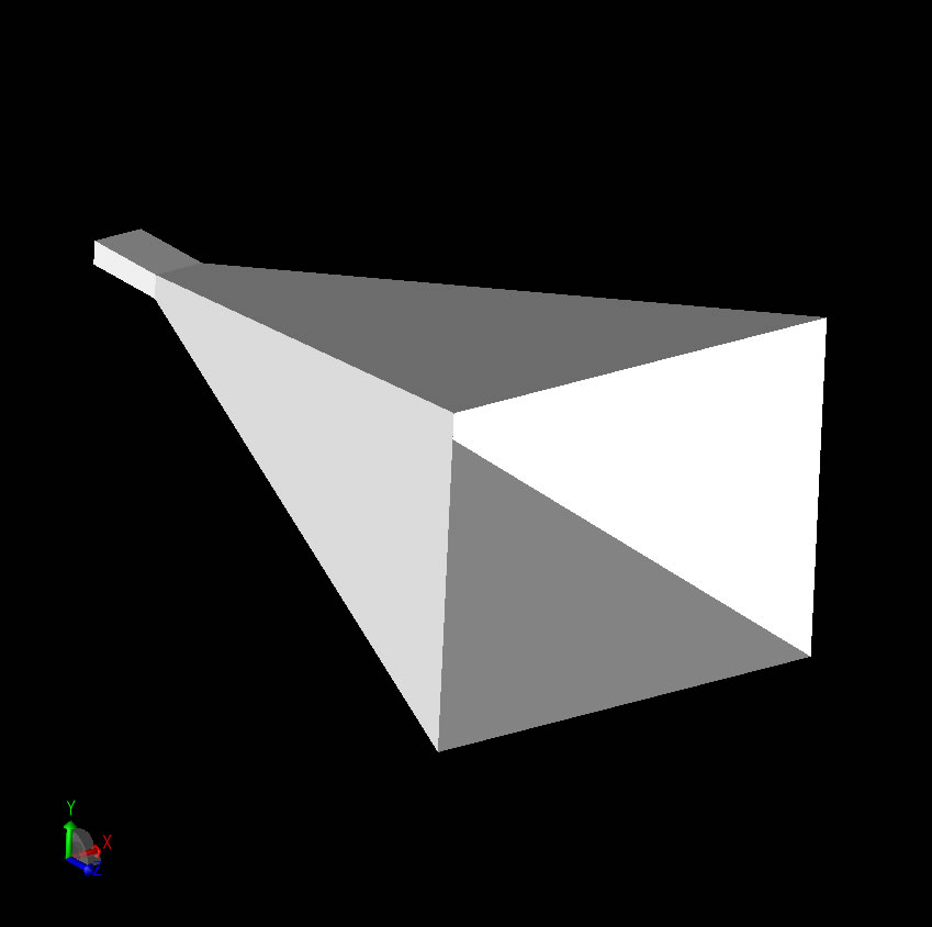
Figure 1: The horn geometry as drawn in the XF.
The desired frequency for this simulation is 9.3 GHz which results in a maximum grid size of approximately 3 mm for simulation at 10 cells per wavelength. Due to the tapered shape of the horn, the sides of the horn will not be aligned with the XF grid. This could result in staircasing errors in the simulations. To check this, the simulation is first performed using 3mm cubical cells, and then again using 1.5mm cells which should significantly reduce any staircasing error at 9.3 GHz.
The simulation is performed using a standard desktop PC with a single CPU and with an hardware accelerated GPU card. At 3mm resolution, the simulation reaches convergence in seconds on the GPU card. The results show a peak gain of 21 dB with E-plane beamwidth of 9.3 degrees and H-plane beamwidth of 13.6 degrees. These results are close to the theoretical design goals, but are likely affected by the staircasing errors. Plots showing the E- and H-plane peak gain and 3dB beamwidth are shown in Figures 2 and 3.
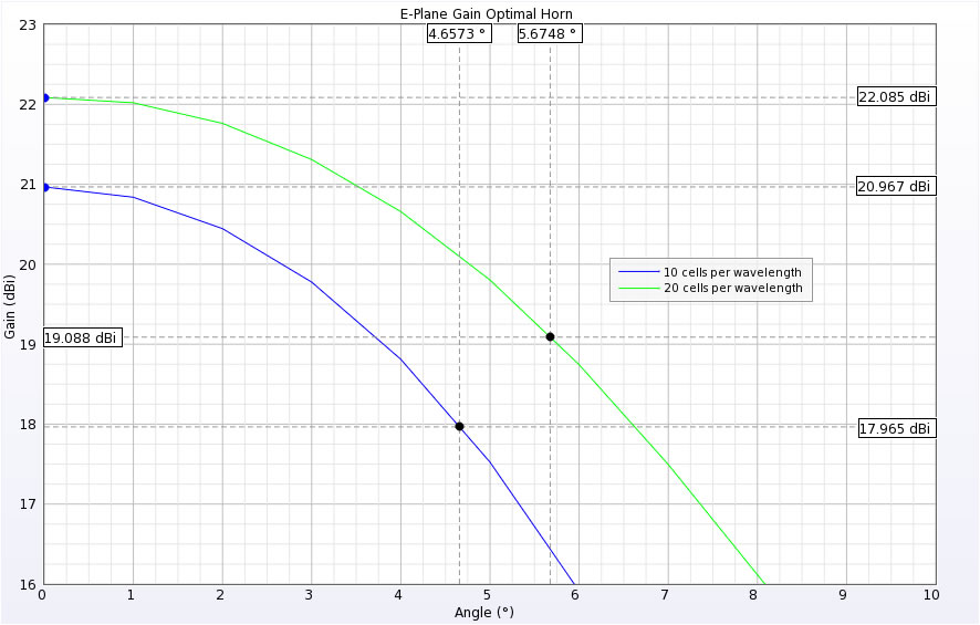
Figure 2: E-plane peak gain and 3dB beam width points.
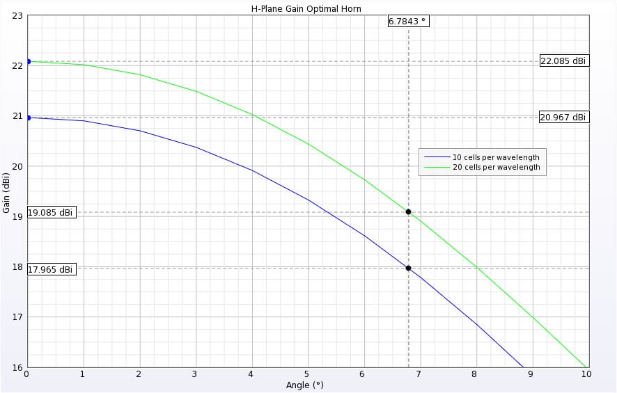
Figure 3: H-plane peak gain and 3dB beam width points.
When the mesh resolution is set to 1.5mm, the simulation converges in under 30 seconds on the GPU card and yields results of peak gain 22.1 dB, and E- and H-plane beamwidths of 11.3 and 13.6 degrees which closely match the theoretical values. Polar plots of the gain in the E- and H-planes are shown in Figures 4 and 5. A run time comparison on the 1.5mm resolution simulation showed a 35x speedup of the GPU over the CPU.
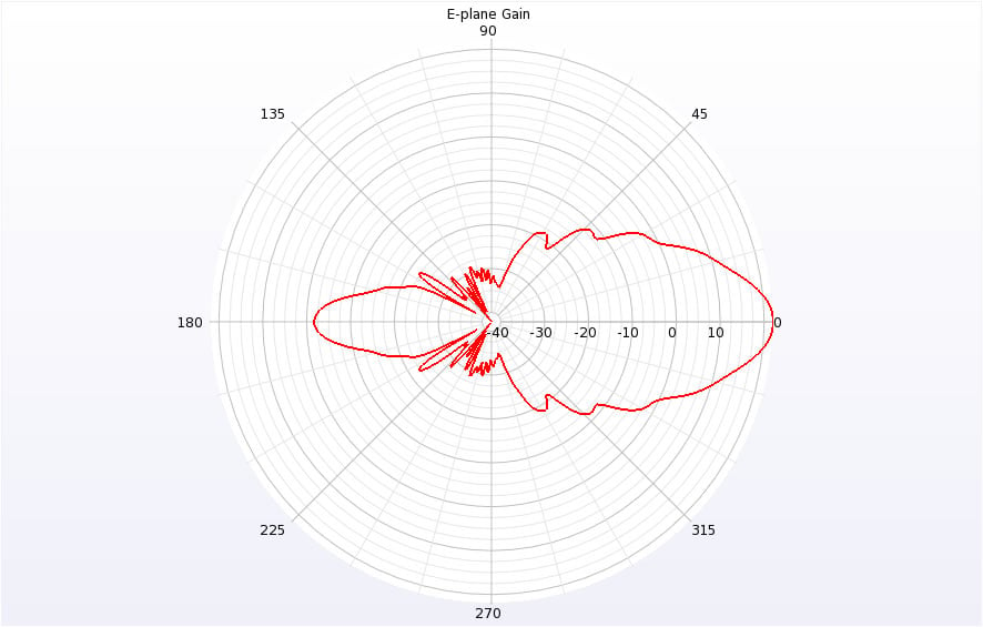
Figure 4: A polar plot of the entire E-plane gain is shown to illustrate the sidelobes and directivity of the horn.
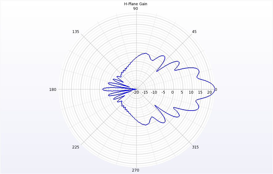
Figure 5: A polar plot of the entire H-plane gain is shown to illustrate the sidelobes and directivity of the horn.
In Figure 6, time-domain near zone electric fields are shown in the two principal planes to illustrate the propagation characteristics of the fields in the horn and to display the diffraction of the fields around the edges of the horn.
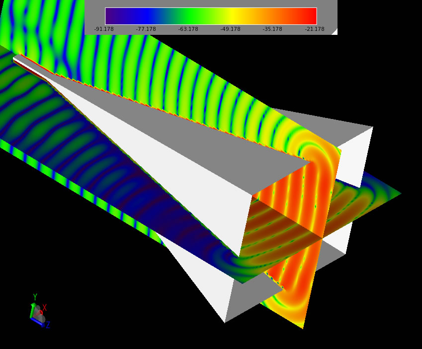
Figure 6: Time-domain electric fields in the principal planes of the horn.
Reference
-
Stutzman and Thiele. Antenna Theory and Design. New York: John Wiley & Sons, 1981.