The IEEE has set standards for RF energy exposure that define the maximum allowable amount and duration of exposure for personnel in controlled and uncontrolled environments. The standard for Maximum Permissible Exposure (MPE) can be viewed in detail in the IEEE C 95.1-2005 document; the term MPE is equivalent to the term Permissible Exposure Limit (PEL) in the previous version of the standard and in other documents and standards. Wireless InSite’s X3D model can be used to estimate whether a particular high-power EM source, whether stationary or moving, can present a hazard to personnel. This information is vital to planning scenarios where high-power sources will be used. Wireless InSite can predict zones within the scene that are considered radiation hazard zones.
Wireless InSite determines the MPE level by direct calculation of the EM quantities used by the standard. It calculates the degree of exposure based on the specific thresholds for the source frequency, the specified environment type, and the time of exposure. Since the standard for MPE includes an exposure time, Wireless InSite considers two possible types of sources: a single stationary source and a moving source (trajectory). The speed at which a moving source traverses the scene can have a noticeable effect on the levels of exposure reported by receivers in the scene. For example, if a transmitter is moving at 1m/s, it would mean the exposure level on the area would be greater than if it was moving at 10m/s. The slower speed results in a longer duration of time where the fields from the antenna are interacting with the study area.
This example discusses how to set up a MPE calculation scenario within Wireless InSite, define the IEEE standard of interest, and review results. The first step is to define the scenario within Wireless InSite. In this example, the Rosslyn city file and terrain file that comes with the software will be used. These files are text-based formats that define the building locations, building heights, terrain vertices and material properties. Figure 1 depicts the Rosslyn City and Terrain file after it has been opened within the Wireless InSite GUI.
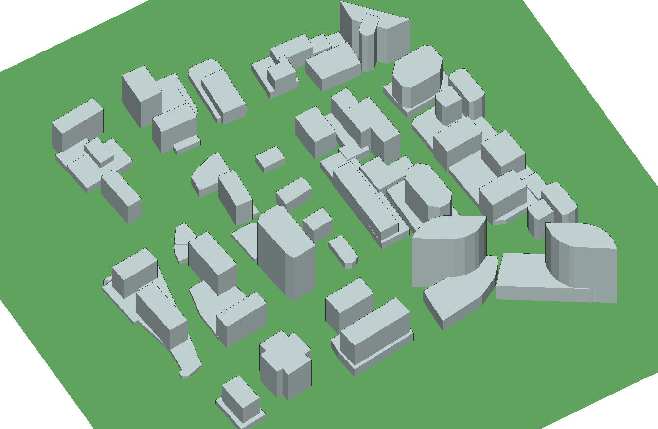
Figure 1: Rosslyn city and terrain file within the Wireless InSite GUI.
The next step is to define a waveform for the MPE scenario. In this case, we will define a 100 GHz sinusoid waveform utilizing the built-in waveforms within Wireless InSite. The software provides a full library of waveforms to use and contains a user-defined format for waveforms. Once the waveform is defined we can define an antenna to assign to our transmitter and receiver locations. Just like the waveforms, Wireless InSite provides a vast library of built-in antenna definitions for use as well as a user-defined antenna format. For this scenario, we will define a horn antenna for the transmitters and an isotropic antenna for the receivers.
Following the definition of the antennas we need to create a transmitter trajectory set which will allow us to define the transmitter’s path of movement throughout the city. Once the trajectory set is defined, the movement start time and speed can be defined under the Advanced Menu within the transmitter properties window as seen in Figure 2. In this case, we will set the velocity as 1 m/s for the velocity and 0 seconds for our start time. The input power for this transmitter has been set to 90 dBm or 1000000 W to represent a high power transmitter. Figure 3 shows the trajectory set within the city of Rosslyn, which defines the transmitter’s path. The receiver set is a defined to be a grid covering the whole city. We will also define a second trajectory set at the same location as the first trajectory set that is moving at 10m/s.
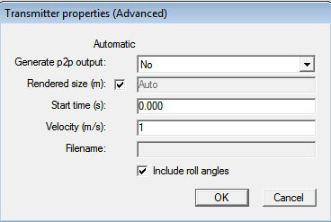
Figure 2: Advanced Menu to set the speed of trajectory path.
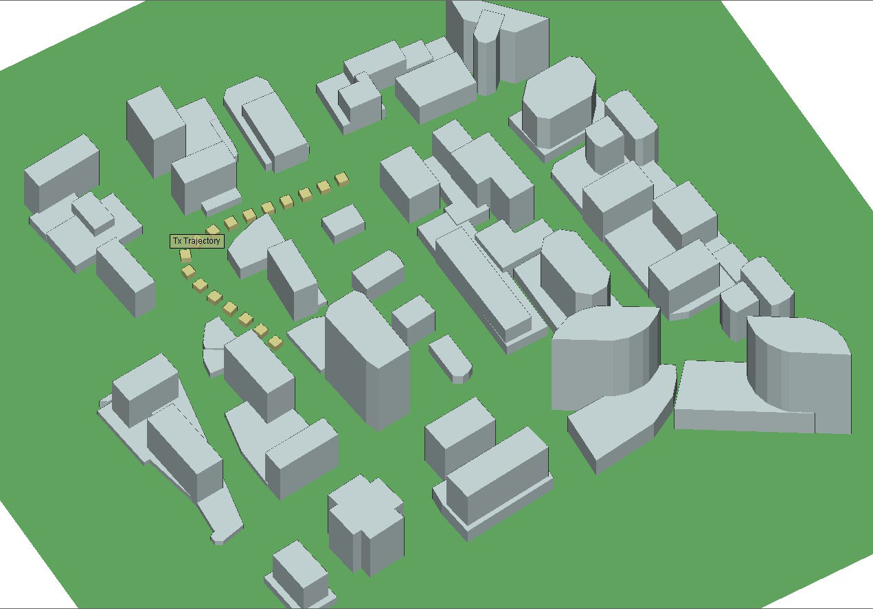
Figure 3: Trajectory within the city of Rosslyn.
After defining the transmitters and receivers, we need to define the study area, which determines the bounds of our calculation space. This is also where the IEEE standards that are used for the MPE calculations are defined. X3D is chosen in the study area properties window as seen in Figure 4. X3D is the only model that calculates the MPE results. The interactions are set to 10 reflections, 0 transmission, and 0 diffractions. Click on the MPE Properties button to activate the MPE calculations. This will bring up the MPE Calculations Window as seen in Figure 5. For this scenario, we will choose IEEE Controlled as the standard to use.
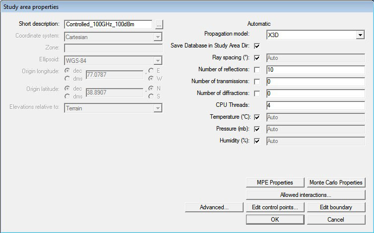
Figure 4: X3D study area property window for MPE scenario.

Figure 5: MPE definition window.
The MPE output available is IEEEC95.1-2005: Peak E-field, IEEEC95.1-2005: RMS E-field, IEEEC95.1-2005: RMS H-field, IEEEC95.1-2005: Average Power and IEEEC95.1-2005: Average Power Density. When a single transmitter is used, these outputs can be viewed or plotted as MPE Threshold. If multiple transmitters are used the Aggregated MPE Threshold can also be shown. Figure 6 shows IEEEC95.1-2005: Average Power Density MPE Threshold for the first trajectory set moving at 1m/s and Figure 7 shows IEEEC95.1-2005: Average Power Density MPE Threshold for the second trajectory set moving at 10m/s. The area in red signifies a hazard zone at or above 100% exposure. The yellow zone represents an exposure rate of between 51% and 100%. The green represents an exposure rate of between 0% and 50%. Comparing the figures, Figure 6 shows more hazardous areas due to the increase in exposure time caused by the slower transmitter movement speed. The purple means no signal was received at this location.
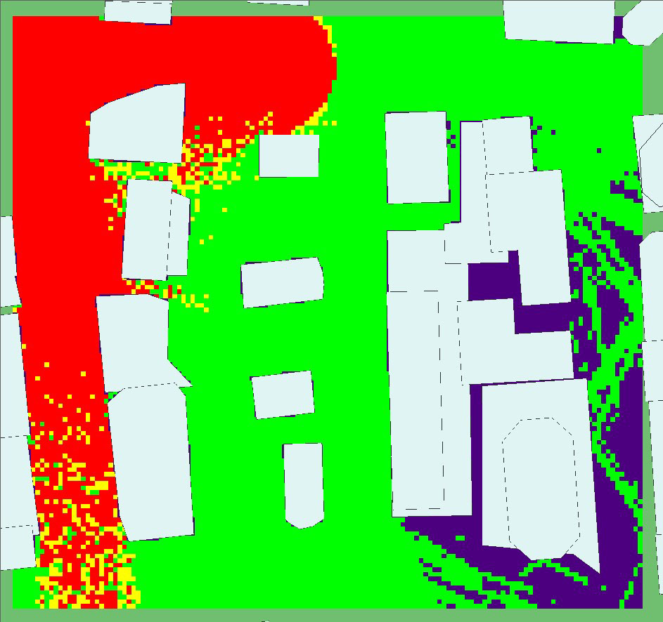
Figure 6: IEEEC95.1-2005: Average Power Density for transmitter set moving at 1m/s.
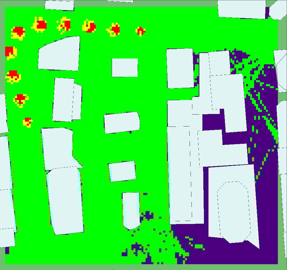
Figure 7: IEEEC95.1-2005: Average Power Density for transmitter set moving at 10m/s.
This example has demonstrated the MPE calculation within Wireless InSite for predicting hazard levels from high-powered RF devices. The hazard level prediction combines the EM analysis from the X3D model, the time of exposure, and the threshold levels set by the IEEE for the specific frequency range and environment type used in the simulation. The results demonstrate that as the transmitter is moving faster through the city, the hazard zones change due to the change in exposure time. More areas are considered hazardous within the scenario when the transmitter is moving at 1m/s compared to the hazard zones predicted with the transmitter moving at 10 m/s. This is vital information when planning a project that involves high powered sources and live personnel. Wireless InSite provides an effective way to predict and display the hazardous zones within a scenario using the MPE calculations. These zones let everyone involved know where people can safely stand while the high powered RF source is active. With just a few clicks of the mouse, the project planners can use Wireless InSite to ensure the safety of personnel.