One of the most powerful features of Wireless InSite® is the ability to apply state-of the-art models and analysis methods to a wide range of propagation problems. This example shows the use of the “Urban Canyon” model to make urban propagation predictions in a microcellular environment in a section of Helsinki, Finland. The simulation is compared to the measurements and analysis from the recent paper "Fast Two-Dimensional Diffraction Modeling for Site Specific Propagation Prediction in Urban Microcellular Environments" by W.Zhang, IEEE Transactions on Vehicular Technology, March 2000 [1]. The coverage area studied in [1] as well as this example is shown in Figure 1. It is near a region in Helsinki known as “Senate Square” in position E.
To simulate the propagation characteristics of this portion of Helsinki, the user starts by drawing each building footprint using the “city editor” in the Wireless InSite user interface (shown in Figure 2) or by importing a DXF format model of the city. Using the city editor is a simple procedure of clicking on the boundaries of each building paying attention to scale and building detail. For urban propagation modeling using the “Urban Canyon” model, no building height information needs to be stored; all buildings are considered much higher than the transmitter or receiver locations allowing for uniform building height of, say, 50 meters. After the building has been entered, WI can render 2d as well as 3d in orthographic and perspective views of the city. Figure 3 is a 3d orthographic view of the section of Helsinki to be modeled.
![Figure 1 . The coverage area studied in [1] as well as this example. It is near a region in Helsinki known as “Senate Square” in position E.](https://www.remcom.com/hubfs/Imported_Blog_Media/image-asset-Apr-03-2023-08-57-01-1932-PM.gif)
Figure 1: The coverage area studied in [1] as well as this example. It is near a region in Helsinki known as “Senate Square” in position E.
Figure 2: City Editor showing the 2D outlines of the buildings in the area under consideration.
Figure 3: 3D view of the Helsinki Urban Canyon model and its surrounding study area.
Without specific knowledge of a particular building’s material parameters, a single material can be used for the entire city such as brick or concrete. For this analysis a uniform building material of concrete was used with a dielectric constant of 5 as was done in [1]. With more detailed information, each building can be assigned different material parameters for each of its faces, i.e. glass, steel, etc. The areas in Figure 1 that are crosshatched are believed to be stairs. To begin this analysis these were removed since they do not satisfy the urban canyon model requirement of vertical surfaces being much higher than the transmitter or receiver locations. It is not clear from [1] how these regions were modeled. To determine the effect of the stairs, simulations can be run with and without this feature.
Once the city has been defined, a terrain is fit to the region in question that also has material parameter settings. For this analysis, a dielectric half space was used for the terrain with dielectric constant 25. Adding the terrain is done by right-clicking in the Features list , then New->Feature->Terrain. The terrain can be automatically fit to the other features (the city in this case) or can be specified by particular region, such as land and water. Changing the material parameters of the terrain is done using the dialog box shown in Figure 4.
Figure 4: Material specification dialog box.
Figure 5: Rx Properties box in the process of defining the route along street AOB
Once this is finished, the receiver list will resemble what is shown in Figure 6. The transmitters are placed in a similar fashion. Figure 7 shows the receiver routes placed in the city including the transmitter at point BS and the terrain. Once the transmitters and receivers are defined an antenna can be associated with each of them. For this study, antennas similar to the ones used in Zhang’s paper [1] were added. A narrow beam directional antenna is used for transmitters, and monopoles for each receiver point. Since the analysis is done in a 2D plane, a vertically polarized omni antenna can be used for receive as well.
![Figure 6. Wireless Insite’s main window under the Receivers tab showing the complete set of receiver routes from [1]. A grid of 3528 receivers was also added which covers the study area to produce a surface plot of received power or path loss. This …](https://www.remcom.com/hubfs/Imported_Blog_Media/image-asset-Apr-03-2023-08-57-02-5484-PM.gif)
Figure 6: Wireless Insite’s main window under the Receivers tab showing the complete set of receiver routes from [1]. A grid of 3528 receivers was also added which covers the study area to produce a surface plot of received power or path loss. This is shown in the last line.
Figure 7: Project view showing receiver routes and transmitter.
Figure 8: Main window with Antenna tab clicked. In this window both antennas for 900.5 and 1800 MHz are shown.
Next the Study Area is added to completely enclose the city. Initially, the calculation is done with the Urban Canyon ray-shooting model with 4 reflections, 2 diffractions and fully correlated. Properties of the other parameters of the calculation are all available from the Wireless InSite’s main window by selecting the appropriate tab and right-clicking on the item. For the initial run all receivers in the project are active or in use. For the purposes of detailed study, on a particular street or subdivision, receiver sets which are outside the area of special interest can be made inactive to shorten the run time. Running a simulation: The project is now ready to make calculations for the transmitter and receiver locations shown in Figure 7. After saving all files with an appropriate file name, right-clicking Project>Run>New will launch the calculation engine. Once the calculation is finished, comparisons can be made to the results found in [1]. The path loss or the received power can be plotted versus distance or receiver number for each if the receiver routes defined. The route along street AOB is shown in Figure 9 and for street KDC in Figure 10. The analysis can be made at several frequencies in a single run. The path loss prediction along LMN at 1.8 GHz is shown in Figure 11.
![Figure 9 Plot of Path Loss along street AOB showing the results from Zhang’s [1] analysis and measurements compared to Wireless Insite.](https://www.remcom.com/hubfs/Imported_Blog_Media/image-asset-Apr-03-2023-08-57-01-4802-PM.gif)
Figure 9: Plot of Path Loss along street AOB showing the results from Zhang’s [1] analysis and measurements compared to Wireless Insite.
![Figure 10. Plot of Path Loss along street KDC showing the results from Zhang’s [1] analysis and measurements compared to Wireless Insite.](https://www.remcom.com/hubfs/Imported_Blog_Media/image-asset-Apr-03-2023-08-57-01-7455-PM.jpeg)
Figure 10: Plot of Path Loss along street KDC showing the results from Zhang’s [1] analysis and measurements compared to Wireless Insite.
Figure 11: Path loss comparison at 1.8 GHz along street LMN.
The Wireless InSite results cannot reproduce the small-scale fades of the measurements since the building locations and shapes are not known with great accuracy. Given this, the agreement is quite good. If more accurate building data were available receiver routes could be placed with receivers at every 50 cm or so and the correlated complex electric fields saved (an available option by clicking Advanced in the Receiver properties dialog box).
Another source of error for both the Zhang calculations as well as Wireless Insite is that the measurements were made with some level of traffic in the streets. The effects if buses, trucks, and cars are not present in the calculations but do have a measurable and dynamic effect on the propagation. This is probably most evident near the intersections M,O, and D where line-of-sight (LOS) should dominate if there is no traffic. The under-estimate of the path loss at these locations for both Zhang’s and Wireless InSite’s analysis is partly due to the absence of auto traffic. Some metallic structures (simulating traffic) can be placed in the path to see the effect it has on accuracy. This is shown in Figure 12. The analysis is re-run with the new obstacles and compared to the result without traffic in Figure 13. It is clear that some of the underestimate of the LOS path loss could be due to the absence of traffic.
Figure 12: The rectangular blue structures are added to simulate traffic near the intersection on AOB
Figure 13: Plot showing the difference in path loss prediction when considering the effect of vehicular traffic. The red trace shows the path loss near the junction with no traffic present and the blue trace shows the increase in path loss due to the few fictitious vehicles from Figure 12.
To analyze the effect of the steps around DEF in Figure 1 (crosshatch), The model can be run with and without sub-structure defining the steps. Individual runs can be made to study the street BC area. The individual ray paths can be viewed to gain insight into the propagation mechanisms involved in a given area. The ray path analysis made without steps is shown in Figure 14 and with steps in Figure15.
Figure 14 . Studying the effects of the stairs around Senate Square. The stairs have been removed.
Figure 15 . The propagation down street BC with the stairs present.
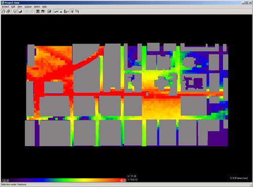
Figure 16 . Surface area plot of the Helsinki received power at 900 MHz.
This was an example of how Wireless Insite can be used for prediction and planning in Urban microcellular environments and the ability to match state-of-art analysis methods to ensure first pass design success. Typically to achieve similar results, the calculation will take a few minutes in a 1 GHz Pentium 4 workstation.
References
- "Fast Two-Dimensional Diffraction Modeling for Site Specific Propagation Prediction in Urban Microcellular Environments" by W. Zhang, IEEE Transactions on Vehicular Technology, March 2000.