Introduction
In this antenna design example, a dual-band antenna constructed of textile material is evaluated for use in a body-worn application. The design and evaluation are taken from a published journal paper [1]. The base antenna design is a rectangular patch constructed of a textile material covered in a conducting tape. The patch has shorting walls and a tuning via to enhance performance and provide dual-band results. The antenna is flexible, so it is simulated in both flat and bent conditions to gauge the impact on performance. Radiation of the antenna over a body phantom is performed to confirm the Specific Absorption Rate (SAR) values are acceptable. For use in MIMO applications, the patch is paired in arrays of varying configurations and evaluated.
Device Design and MIMO Antenna Simulation
Single Antenna - Flat
This MIMO antenna simulation is focused on a flexible dual-band patch antenna design constructed of textile material for use in a body-worn application. The basic antenna design of the patch is shown in Figure 1a (top view) and 1b (angle view). The patch is rectangular and consists of a 3 mm layer of a felt fabric that acts as the substrate which is covered by a thin layer of flexible conductive tape. Two adjacent sides of the substrate are covered with shorting walls to aid in isolation between neighboring elements when used as part of an array. A via is positioned in the substrate to provide a way to modify the resonant modes of the cavity to achieve dual band performance. The design parameters and performance tests mimic those found in the paper [1].
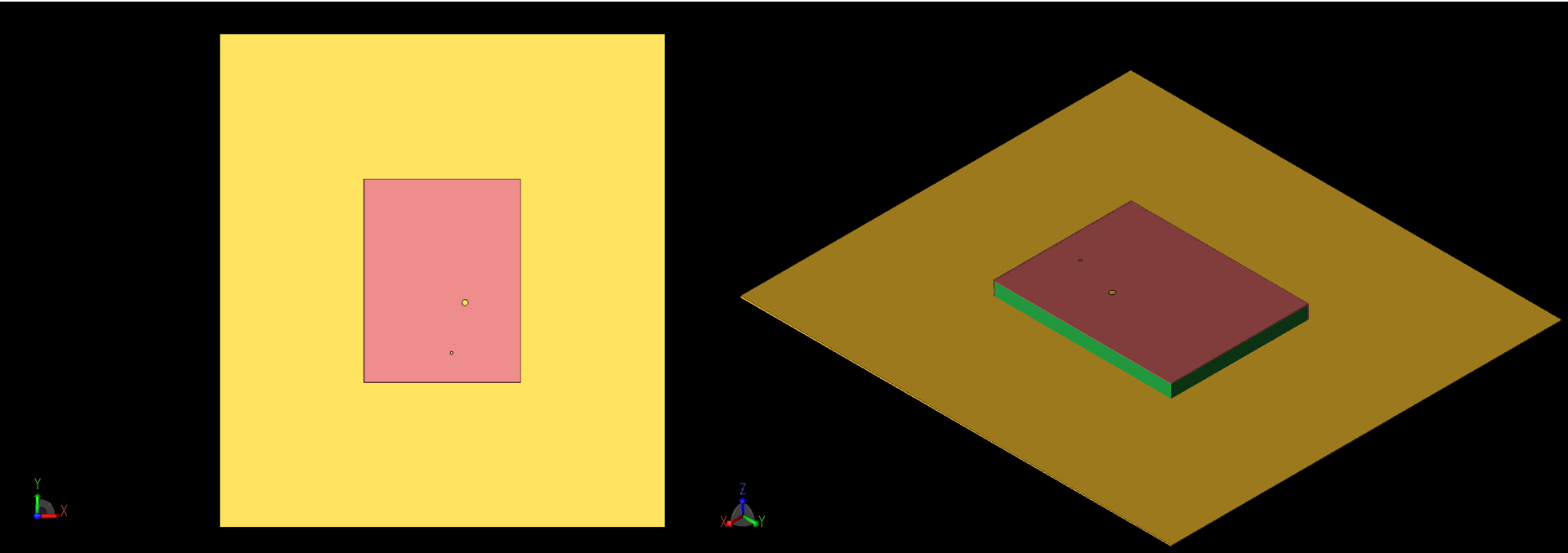
Figure 1: Top (left, 1a) and angled (right, 1b) views of the patch antenna geometry are shown. The coaxial feed and via are visible as large and small circles on the top of the patch. The -X and -Y sides of the patch are shorted to the ground plane.
The initial patch antenna is simulated in XFdtd and the return loss is found to be acceptable in bands around 2.5 GHz and 5.5 GHz with a broader band found at the higher frequency (Figure 2). In Figure 3, the steady-state magnetic field is shown across the surface of the patch at several frequencies. In Figure 3a, the first mode is shown at 2.45 GHz. Other modes are visible at 5.2 GHz (Figure 3b) and 5.8 GHz (Figure 3d). Figure 3c shows the H-fields at 5.5 GHz. The gain pattern for the patch is spherical (Figure 4) and has a peak value of about 3.4 dBi at 2.45 GHz and 6.7 dBi at 5.5 GHz.
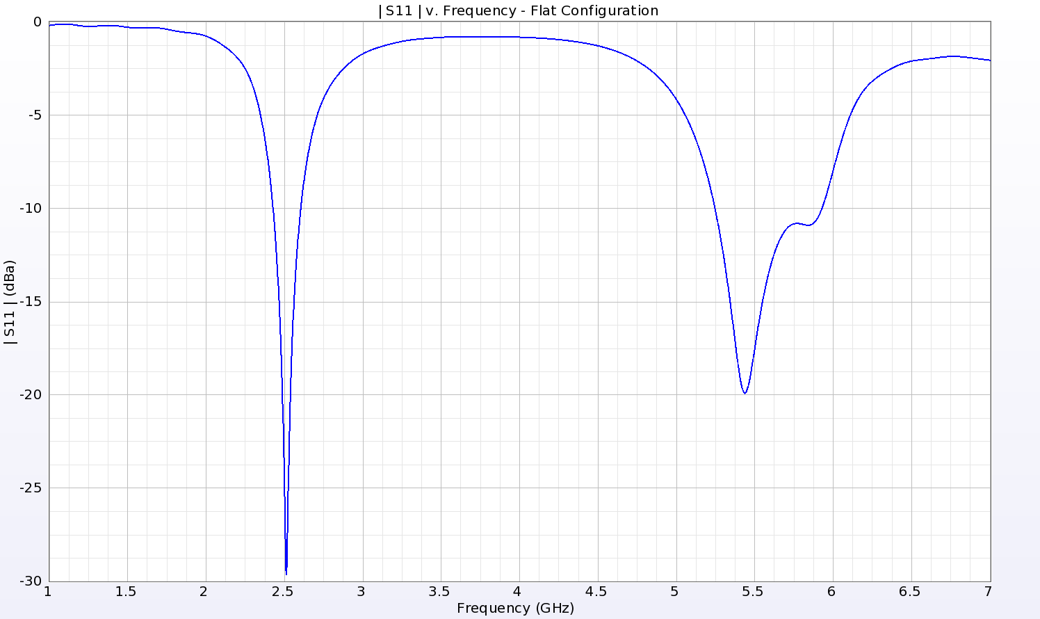
Figure 2: The return loss for the single patch shows a deep null around 2.5 GHz and two shallower nulls around 5.4 and 5.8 GHz which produce a broader operating region at the higher frequency bands.
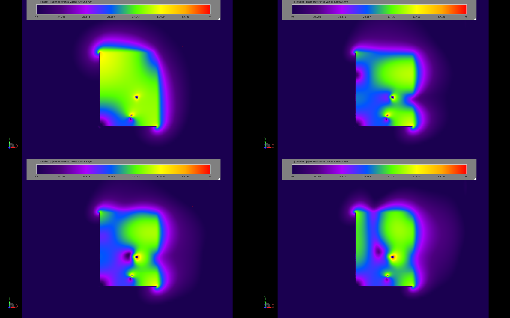
Figure 3: Plots of the steady state magnetic field distribution show the different operating modes of the patch. The top left image (3a) is at 2.45 GHz while the top right (3b) is at 5.2 GHz. The bottom two images (3c and 3d) show the response at 5.5 and 5.8 GHz.
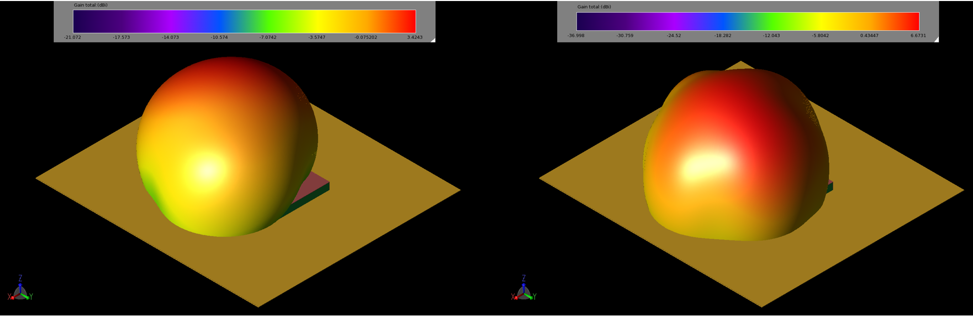
Figure 4: The gain patterns of the patch at 2.45 GHz (left, 4a) and 5.5 GHz (right, 4b) are spherical with peak gain values of 3.4 and 6.7 dBi, respectively.
For evaluation of the SAR performance, the patch is placed 5mm above a layered phantom consisting of skin, fat, and muscle layers displayed in Figure 5. The peak 1-gram averaged SAR levels for 0.5 W input power were computed and found to be 0.113 W/kg and 0.18 W/kg at 2.45 and 5.5 GHz, well below the maximum allowed by standards. Using the 10-gram averaged SAR analysis, the SAR levels for 0.5 W input power were 0.058 W/kg and 0.082 W/kg at 2.45 and 5.5 GHz, again well below the maximum allowed. The distribution of the 10-gram averaged SAR values for each frequency are shown in Figure 6.
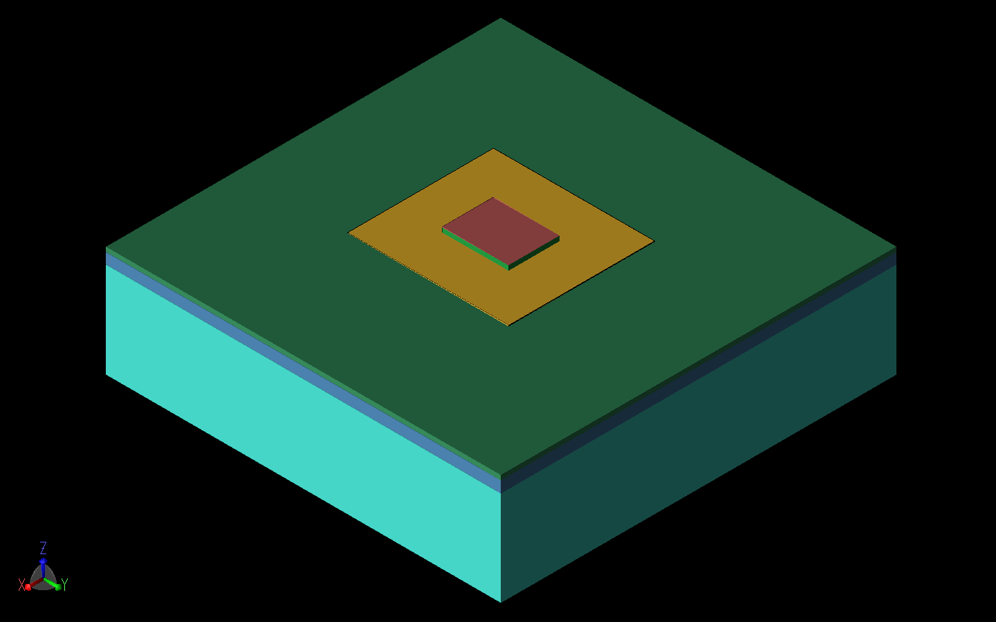
Figure 5: For testing the Specific Absorption Rate (SAR) of the patch antenna, it is simulated above a three-layer phantom of skin, fat, and muscle equivalent tissues.
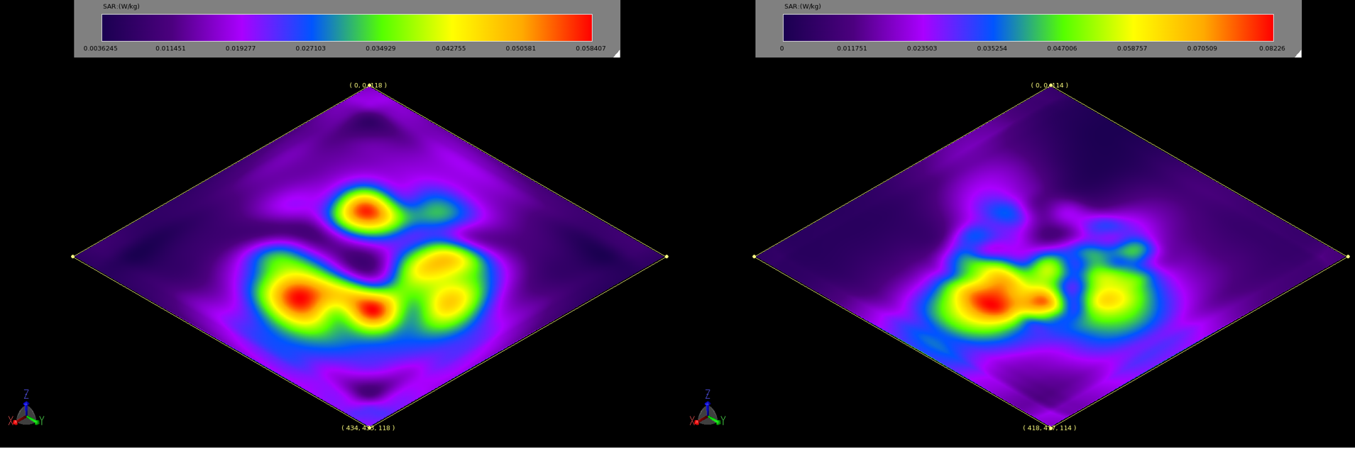
Figure 6: The 10g averaged SAR plots at 2.45 GHz (left, 6a) and 5.5 GHz (right, 6b) indicate the regions with the highest power absorption in the phantom. The values are for an input power of 0.5 W and are well below the allowable standards.
Single Antenna – Curved
The patch antenna design is next evaluated for performance under more realistic conditions for a body-worn setting where there might be curvature of the antenna. The design is tested at bend radii of 40 mm and 80 mm over both the X and Y axes of the antenna. The bending configurations of 40 mm radius in each direction are shown in Figure 7. For all bending cases the return loss performance is very consistent in the lower band while some variation of the null depth and location occurs in the higher band, as shown in Figure 8. In all cases the antenna performance is maintained at acceptable levels. For a 40 mm bend radius, the gain patterns at 2.45 GHz are very consistent with the flat geometry in pattern shape while the maximum gain drops from 3.4 dBi to 2.2 dBi (bend on X axis) and 1.8 dBi (bend on Y axis). At 5.5 GHz the gain pattern becomes less uniform and the peak gain is reduced by about 2 dBi from the flat geometry case. The 40 mm bend radius gain patterns are shown in Figure 9. For the 80 mm bend radius cases the shape of the gain patterns is closer to those of the flat geometry case, but the peak gain is reduced to 2.8 dBi (bend on X axis) and 2.5 dBi (bend on Y axis) at 2.45 GHz. The 5.5 GHz peak gain is reduced by about 1 dBi in both bending cases. The patterns for the 80 mm bend radius cases are shown in Figure 10.
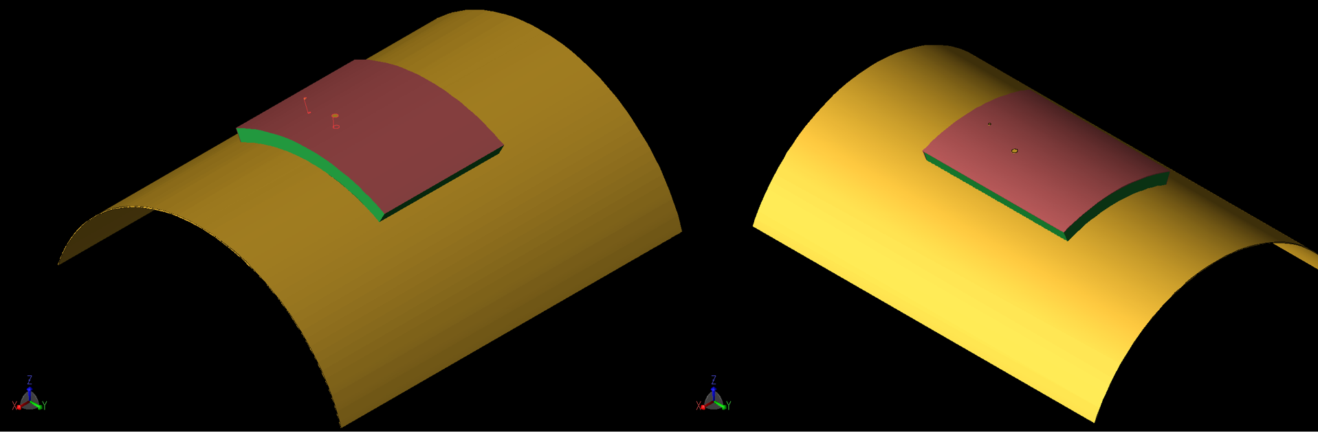
Figure 7: The patch is shown in a curved configuration where the curve radius is 40 mm. At the left (7a) the curvature is around the X axis while at the right (7b) it is around the Y axis. Similar geometries were simulated for a curvature of 80 mm radius.
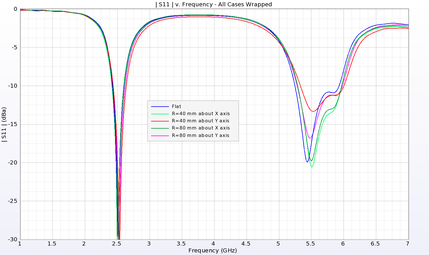
Figure 8: The return loss for all configurations of the patch curved around a radius show similar results, especially at the low end. For the upper resonance, the return loss has slight variations, but the operating region is similar for all cases.
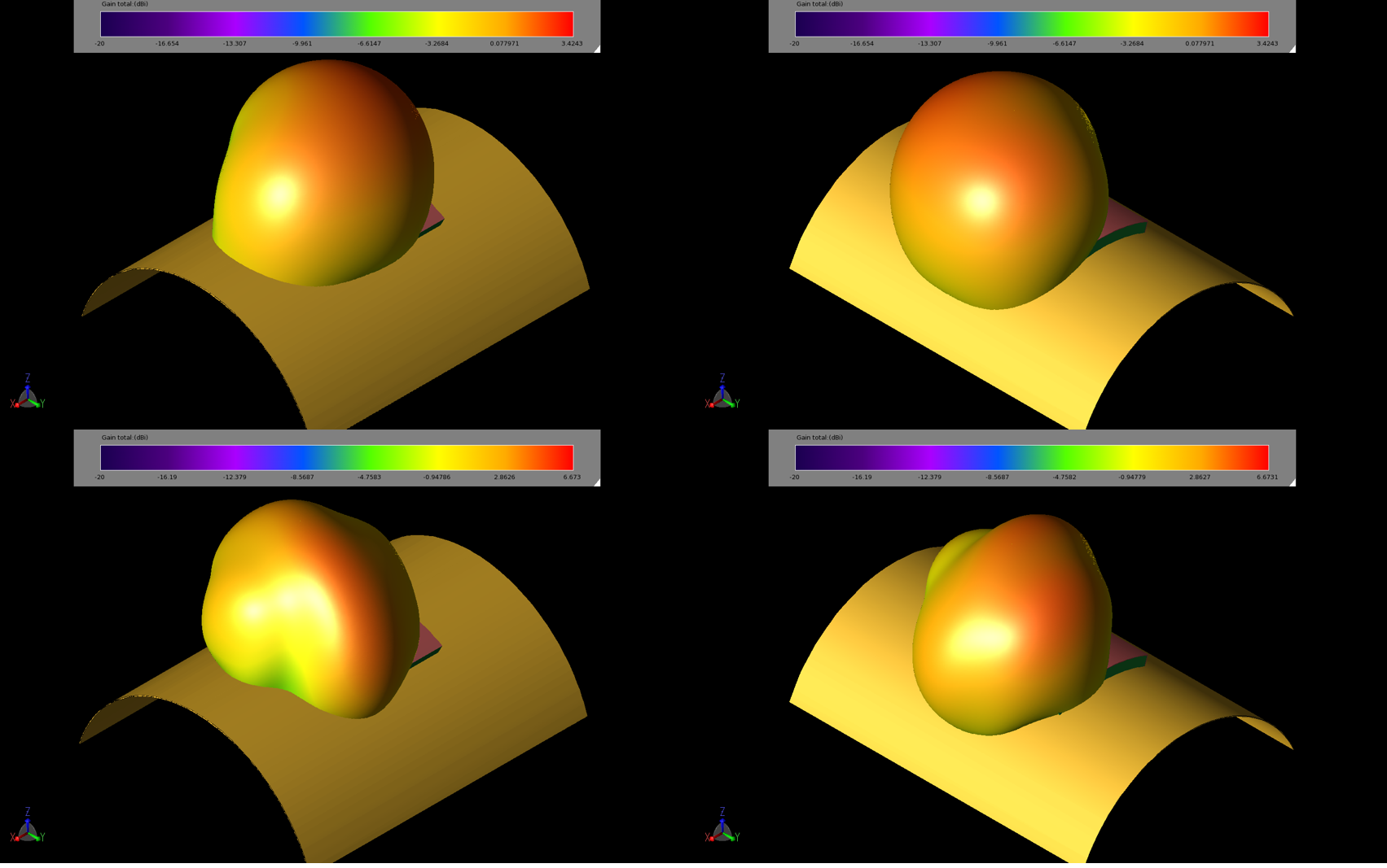
Figure 9: Gain patterns for the patch antenna on the curved structures show slight variations in the patterns and reductions in the peak gain. The images are 40 mm curve about X at 2.45 GHz (upper left, 9a), curve about Y at 2.45 GHz (upper right, 9b), curve about X at 5.5 GHz (lower left, 9c), and curve about Y at 5.5 GHz (lower right, 9d).
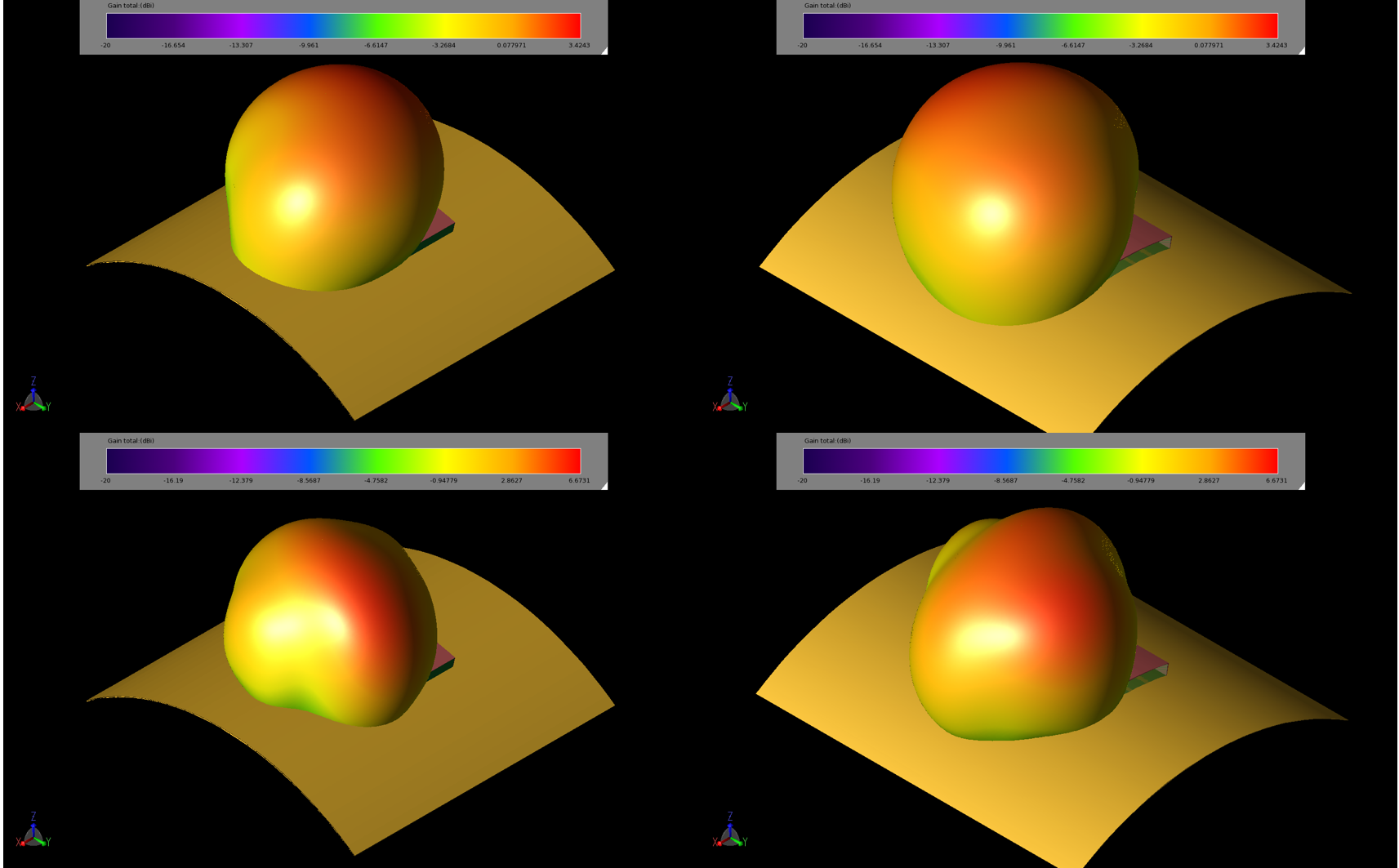
Figure 10: Gain patterns for the patch antenna on the curved structures show slight variations in the patterns and reductions in the peak gain. The images are 80 mm curve about X at 2.45 GHz (upper left, 10a), curve about Y at 2.45 GHz (upper right, 10b), curve about X at 5.5 GHz (lower left, 10c), and curve about Y at 5.5 GHz (lower right, 10d).
MIMO Arrays
The base patch antenna design is next put into a 1x2 antenna array configuration for multiple-input, multiple-output (MIMO) use. The orientation of the two antennas is varied in six different combinations where one or both of the elements is rotated. All configurations have a 10 mm spacing between the antennas, and the edges of the patch that face each other always contain shorting walls to minimize interaction. The six configurations are shown in Figure 11. The return loss performance shown in the antenna array simulation is very consistent regardless of the orientation of the second element, as shown in Figure 12. The interaction between the elements, determined by the S12 parameter, stays below -17 dB (Figure 13).
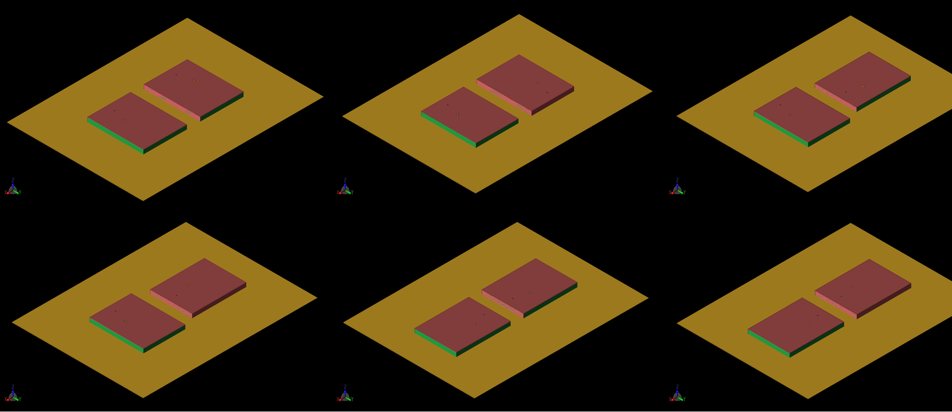
Figure 11: Six configurations of a 1x2 MIMO array were evaluated for performance. In each case, the separation between antenna elements is 10 mm and a shorted side is always facing the adjacent element. The configurations are labeled a, b, and c across the top row and d, e, and f across the bottom. In each case there is some rotation of the elements to change the location of the feed points and the shorting walls.
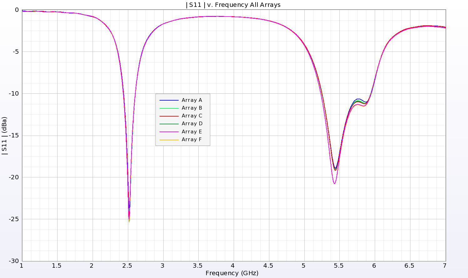
Figure 12: The return loss from all variations of the MIMO array (a through f of Figure 11) are nearly identical.
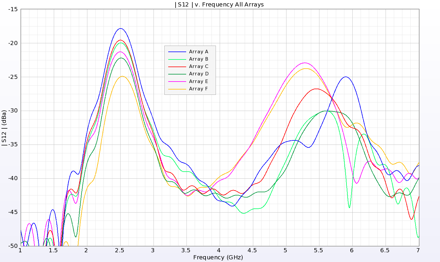
Figure 13: The isolation between the two elements of the MIMO array is demonstrated by the plot of S12 magnitude. For all cases, the isolation remains less than -17 dB.
The individual gain patterns for the various configurations shown in Figure 11 are computed separately and found to have similar pattern shape and peak gain such as those shown in Figure 14. The interaction of the two patterns is considered by computing the Envelope Correlation Coefficient and the Complex Correlation Coefficient to determine if the arrays have acceptable diversity. The coefficients for all array configurations are well below the 0.5 value considered acceptable and are detailed in Table 1.
Table 1: Envelope Correlation and Complex Correlation Coefficients for the six MIMO arrays at 2.45 and 5.5 GHz.
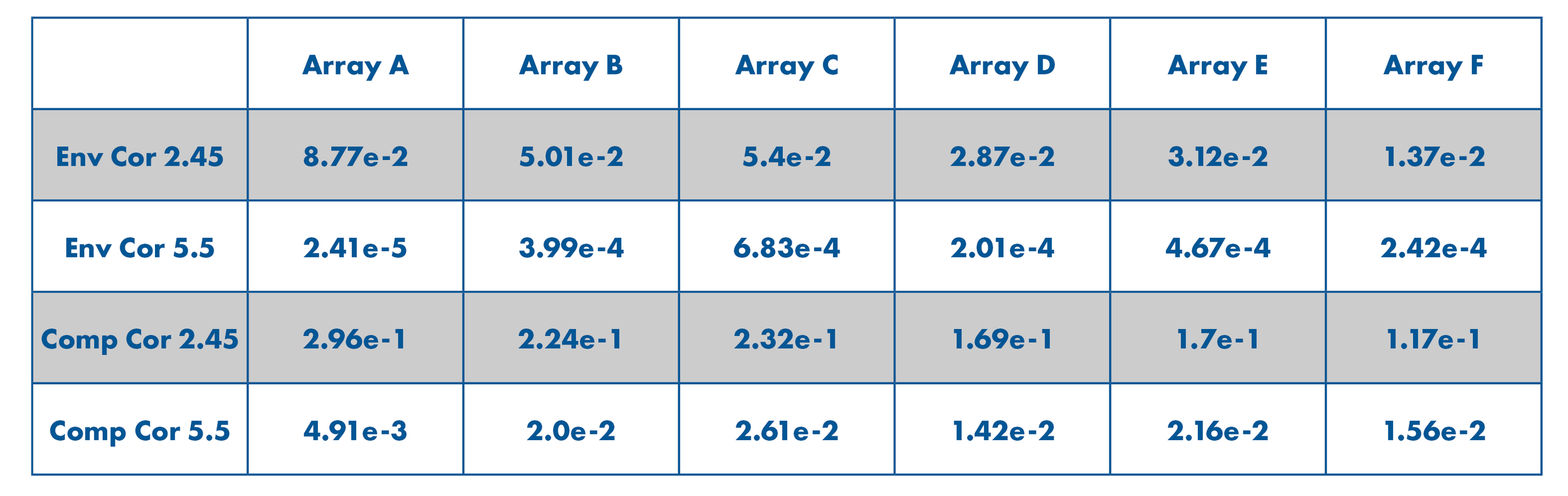
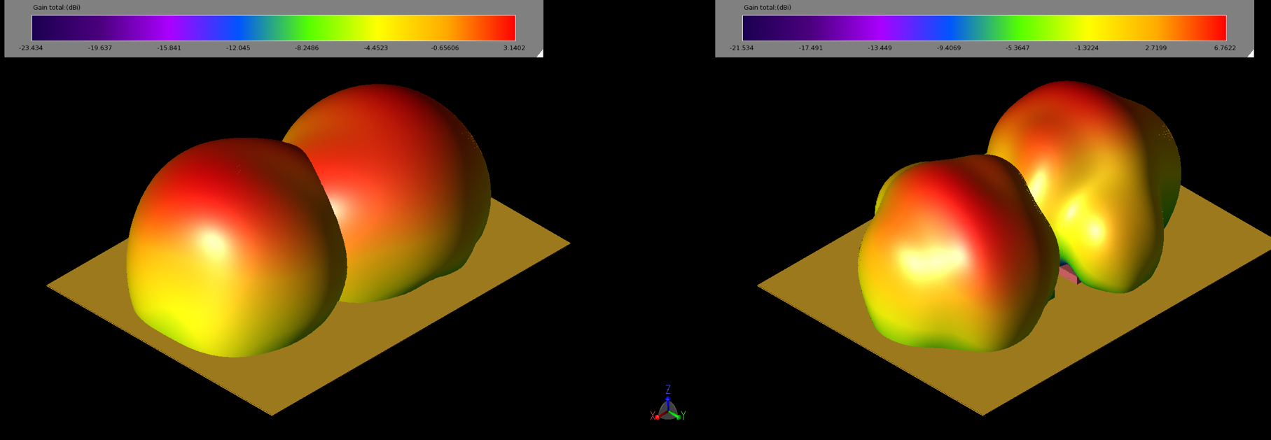
Figure 14: The gain plots of each patch for configuration 11b are plotted at 2.45 GHz (left, 14a) and 5.5 GHz (right, 14b). These plots are for each antenna active independently.
To gauge the coverage of the array, the equivalent (or effective) isotropic radiated power (EIRP) is commonly used as a measure. Using the configuration of Figure 11b, the cumulative distribution function of the EIRP is plotted and marked for an input power of 23 dBmW in Figure 15. The graph indicates a coverage of (1 – 0.69755) or 30.2% of the sphere at 2.45 GHz and (1 – 0.62423) or 37.6% of the sphere at 5.5 GHz. The six configurations of Figure 11 averaged a coverage of 28.6% at 2.45 GHz and 38.3% at 5.5 GHz.
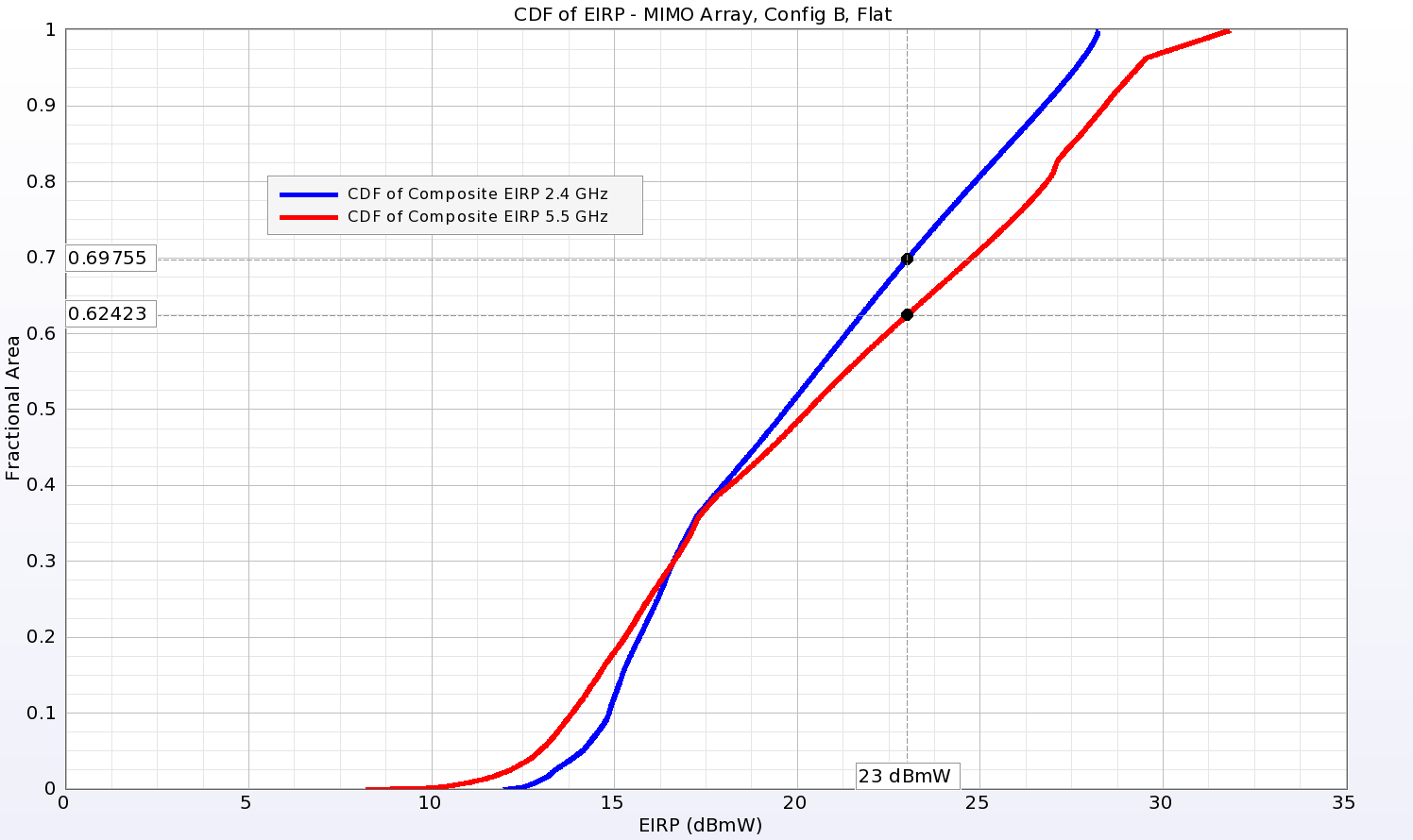
Figure 15: The cumulative distribution function of the Equivalent Isotropic Radiated Power (EIRP) indicates the coverage possible from the array for a given input power. For the array of Figure 11b, the coverage is 30.2% at 2.45 GHz (1-0.69755) and 37.6% at 5.5 GHz (1-0.62423) when an input power of 23 dBmW is chosen.
MIMO Array - Curved
The MIMO array of Figure 11b is next curved around a 40 mm radius as was done for the single patch case previously. The array is shown curved around the Y axis in Figure 16. Following simulation, the S-parameters show good return loss for both antennas and better than -27 dB isolation between the elements across the frequency range (Figure 17). The individual gain patterns for the two curved elements at 2.45 GHz and 5.5 GHz show similar pattern shapes but reduced gain compared to the flat orientation (Figure 18). The envelope correlation coefficient for the curved array is very good at 6.0e-3 for 2.45 GHz and 5.1e-5 for 5.5 GHz. The complex correlation coefficient is 7.8e-2 and 7.1e-3 for the same frequencies. In the EIRP analysis, the coverage of the curved array for an input power of 23 dBmW improves over that of the flat array with values of 32.2% and 48.1 % for 2.45 and 5.5 GHz, as shown in Figure 19.
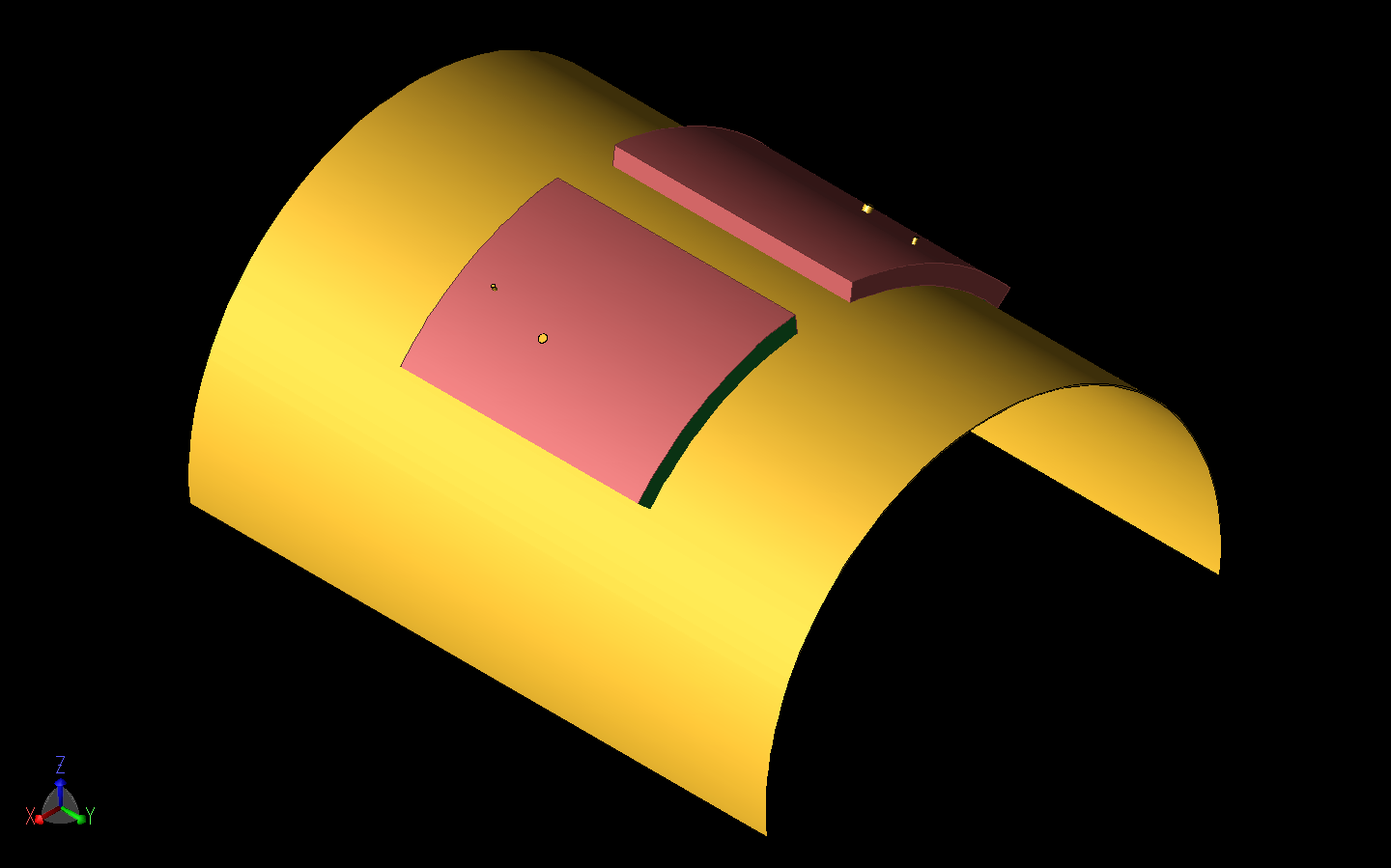
Figure 16: The MIMO array from Figure 11b is shown curved around a cylinder of radius 40 mm about the Y axis.
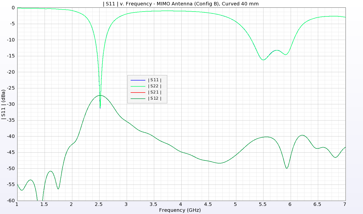
Figure 17: The return loss and isolation from the curved MIMO array of Figure 16 shows good performance with bands around 2.5 GHz and 5.3-6 GHz.
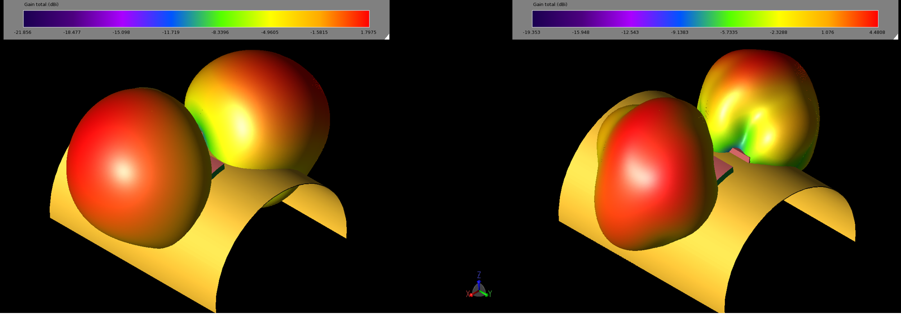
Figure 18: The gain patterns of the array elements for the curved structure of Figure 16 are well separated by the curve and should provide coverage over a broader region.
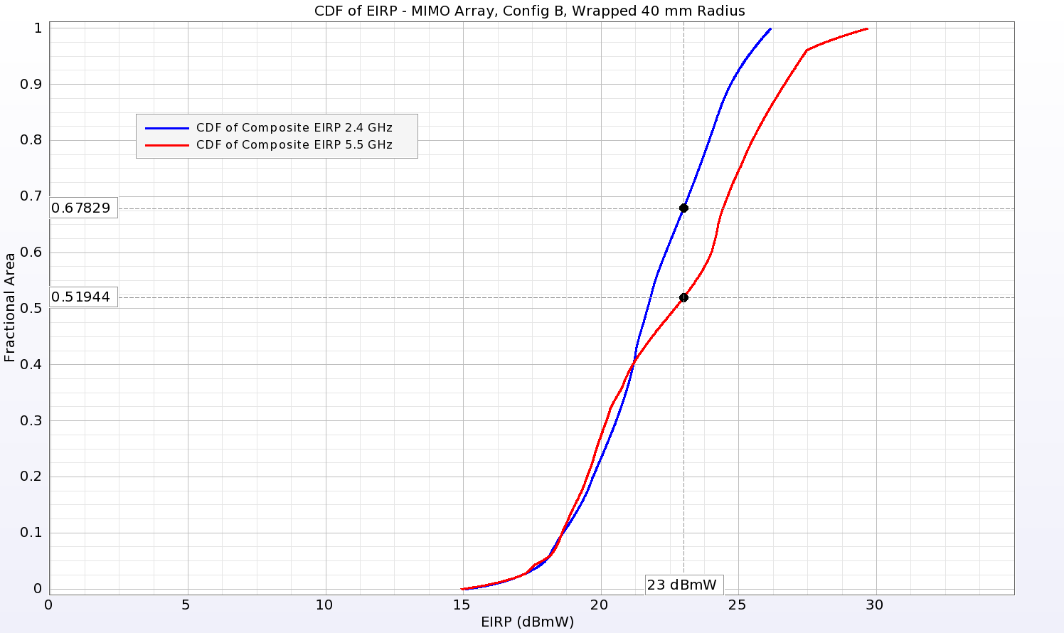
Figure 19: The cumulative distribution function of the Equivalent Isotropic Radiated Power (EIRP) indicates the coverage possible from the array for a given input power. For the array of Figure 16, the coverage is 32.2% at 2.45 GHz and 48.1% at 5.5 GHz for an input power of 23 dBmW which is improved over that for the flat array of Figure 11b.
Conclusion
This example demonstrates a possible wearable antenna design for dual-band use constructed of textile materials. The performance of the antenna remains acceptable as it is deformed as might happen in actual usage cases. When combined in a MIMO array, the antennas show good isolation and acceptable antenna performance.
Reference:
[1] S. Yan, P. J. Soh, and G. A. E. Vandenbosch, “Dual-Band Textile MIMO Antenna Based on Substrate Integrated Waveguide (SIW) Technology,” IEEE Trans. Antennas and Propagation, vol. 63, no. 11, p. 4640-4647, Nov. 2015.