Introduction
This example demonstrates an antenna array simulation for 5G 60 GHz applications of wireless communication for wearable devices such as virtual reality headsets. The antenna design for this example is from the paper [1] by Hong and Choi of Hanyang University. The array is composed of four elements which each have two patches and a parasitic element. The parasitic element aids in producing a wider beam in one dimension to give better coverage. The beams may be steered by varying the phase shift between elements to provide near hemispherical coverage.
Device Design and Simulation
The proposed array design is shown in Figure 1 where the red material represents the substrate (Taconic TLY, relative permittivity of 2.2 and loss tangent of 0.0009) and the green material is Copper. The bottom layer of the antenna is the substrate with a ground plane underneath. This layer is topped by 50-ohm feed lines which then go through impedance matching before reaching the first patch, then a 70-ohm line connects to the second patch. Those patch elements are covered by another substrate layer which is topped by parasitic elements that are perpendicular to the 70-ohm lines. The second layer is visible in the three-dimensional view of the structure in Figure 2. The elements are spaced a half wavelength apart and are fed by Nodal Waveguide ports with variable phase.
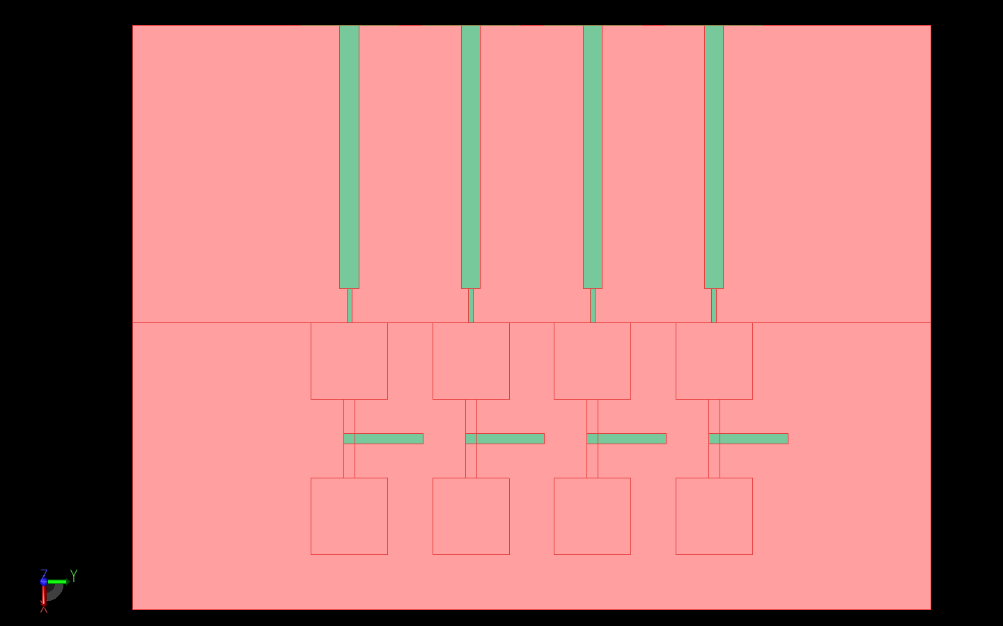
Figure 1: Shown is a top view of the antenna array with the substrate layers shown in red and the metal feed lines and parasitic elements in green. The patches are shown as outlines because they are covered by a second substrate layer.
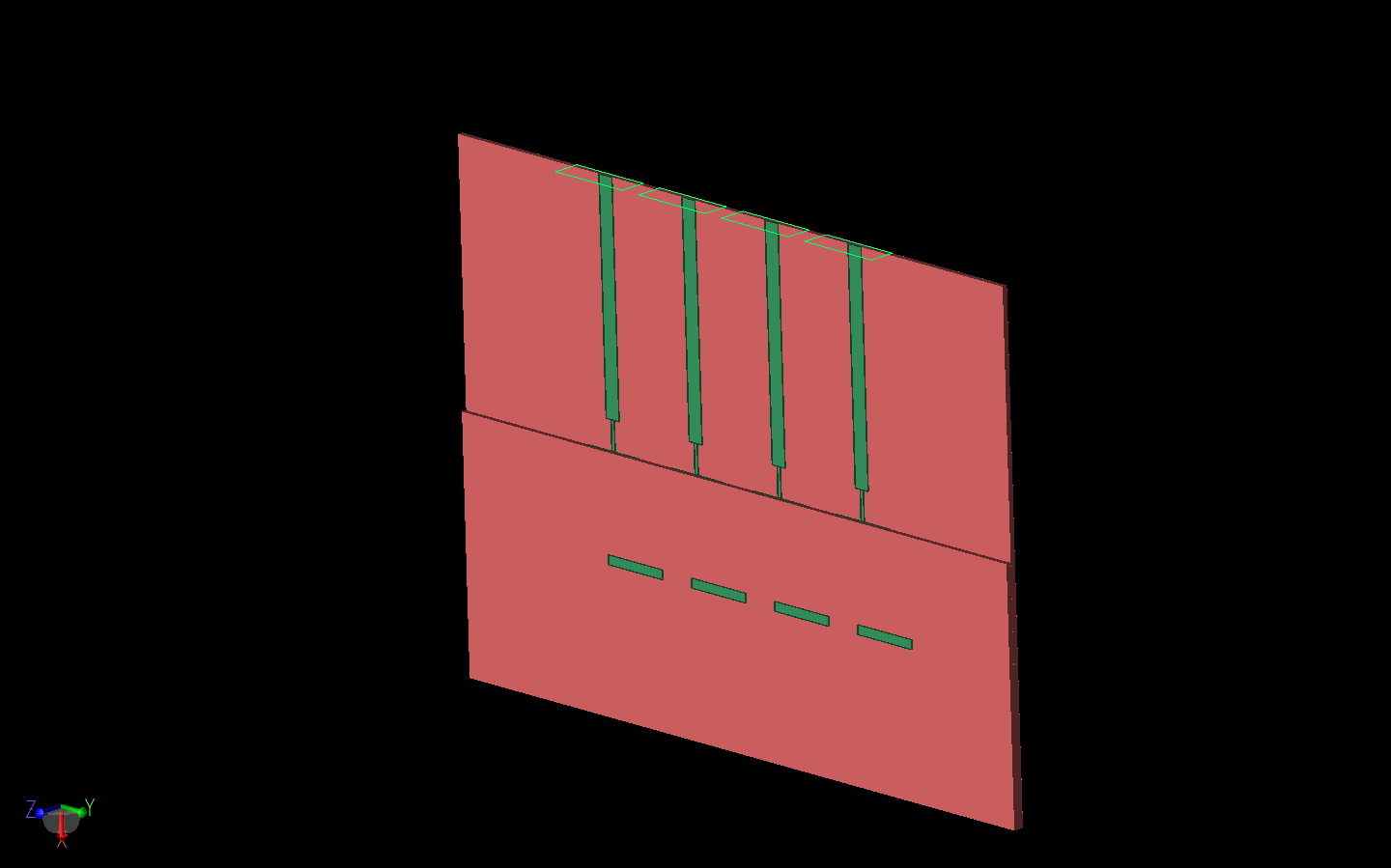
Figure 2: The antenna array is shown in three dimensions with the edge of the top substrate layer more visible over the patches. The four nodal waveguide feed ports are visible on the top of the array.
Initially the antenna array is simulated alone for return loss and gain pattern analysis. For computing S-parameters, each port is simulated individually with the others terminated in a 50-ohm load. The resulting return loss for each port is shown in Figure 3 and the response from each port is quite similar to the others. The simulations are also performed without the parasitic elements to demonstrate the impact of including them on the return loss. As can be seen in Figure 3, the parasitic elements shift the resonance of the antenna higher in frequency and reduce the depth of the S11 null. When the antenna is simulated with all ports active and in phase, the broadside gain pattern is computed as shown in Figure 4. Here it can be seen that without the parasitic element the pattern has deep nulls around +/- 40 degrees which are undesirable. By including the parasitic elements, the nulls are reduced and the array produces a wide fan beam. This beam is better shown in three dimensions in Figure 5 where the pattern can be seen to be broad in the vertical direction and narrow (3-dB beam width of 24 degrees) in the horizontal direction.
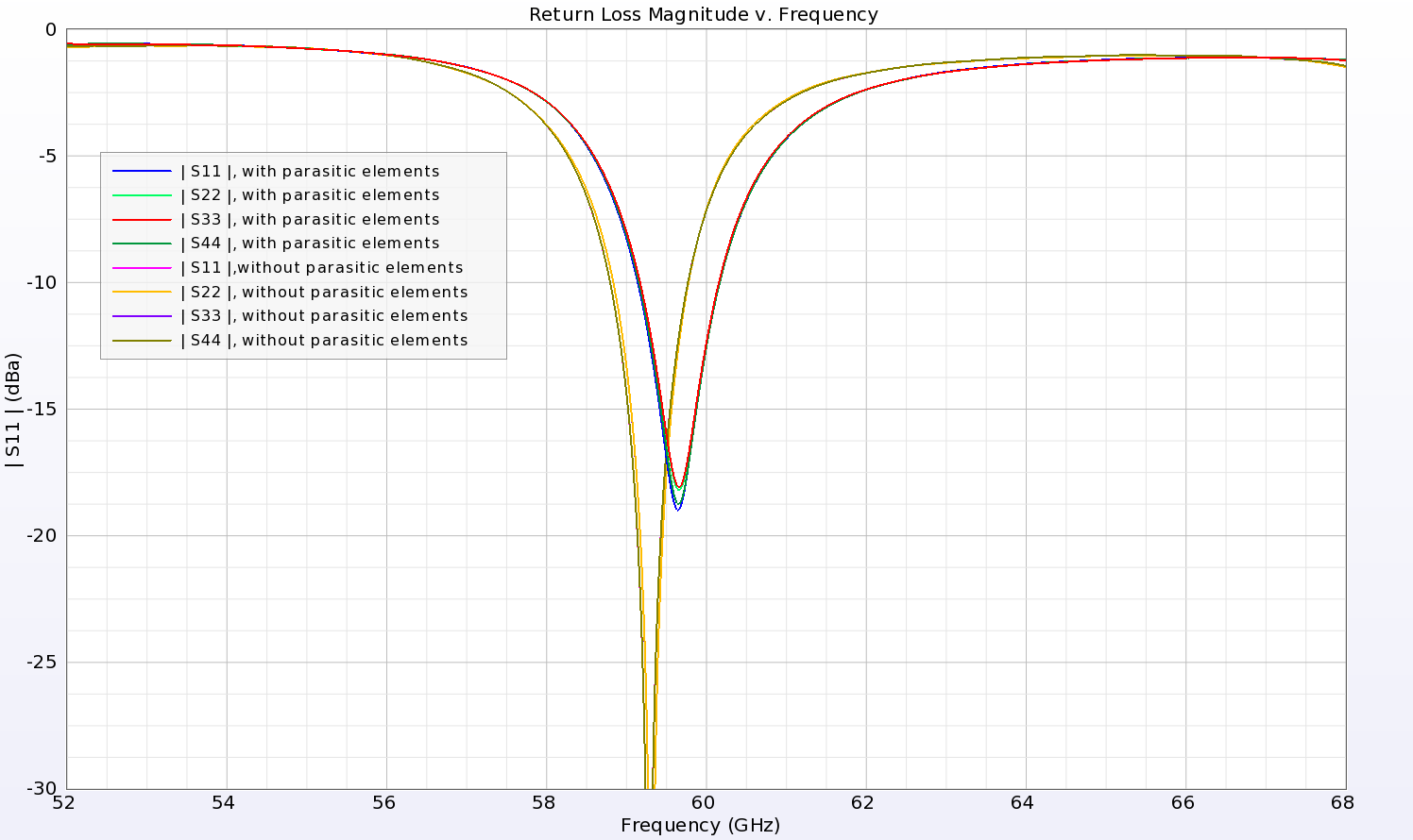
Figure 3: The return loss for each element of the array is quite similar. The addition of the parasitic element shifts the response higher in frequency and reduces the null depth.
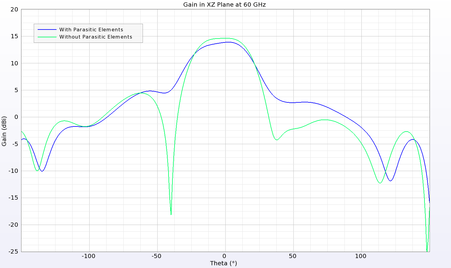
Figure 4: The gain pattern broadside of the array is fairly wide with the parasitic elements included. Without the parasitic elements there are undesired nulls present in the pattern.
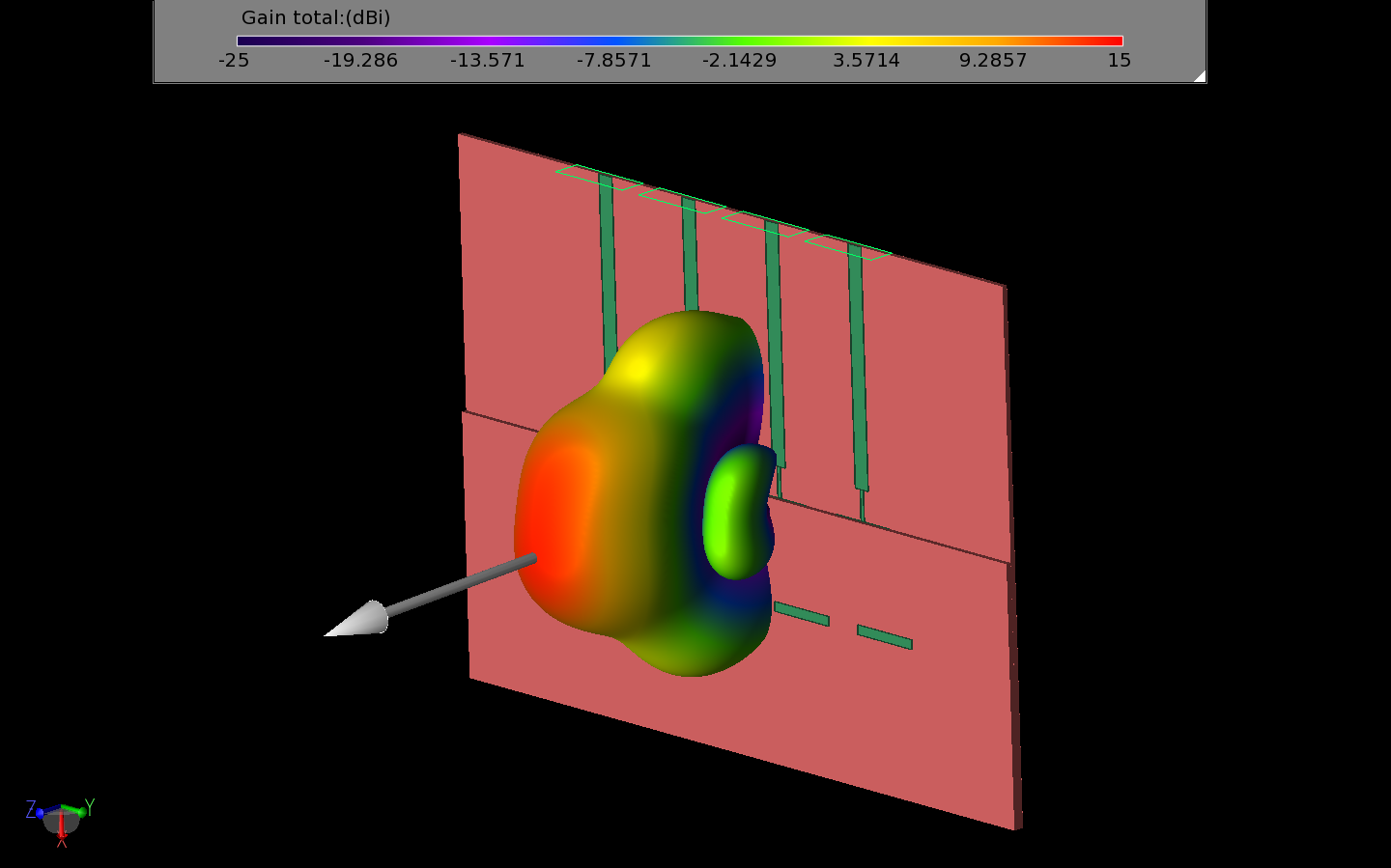
Figure 5: The three-dimensional gain pattern for the equal phase case shows peak gain to the side with a fan shaped pattern.
Beam steering is possible with this array by varying the phasing between the elements. In Figure 6, the array is shown with a beam steered about 30 degrees in the horizontal by applying a phase shift of 90 degrees between the elements. In Figure 7, seven possible beams are shown by varying the phase shift from -90 to 90 in 30-degree steps.
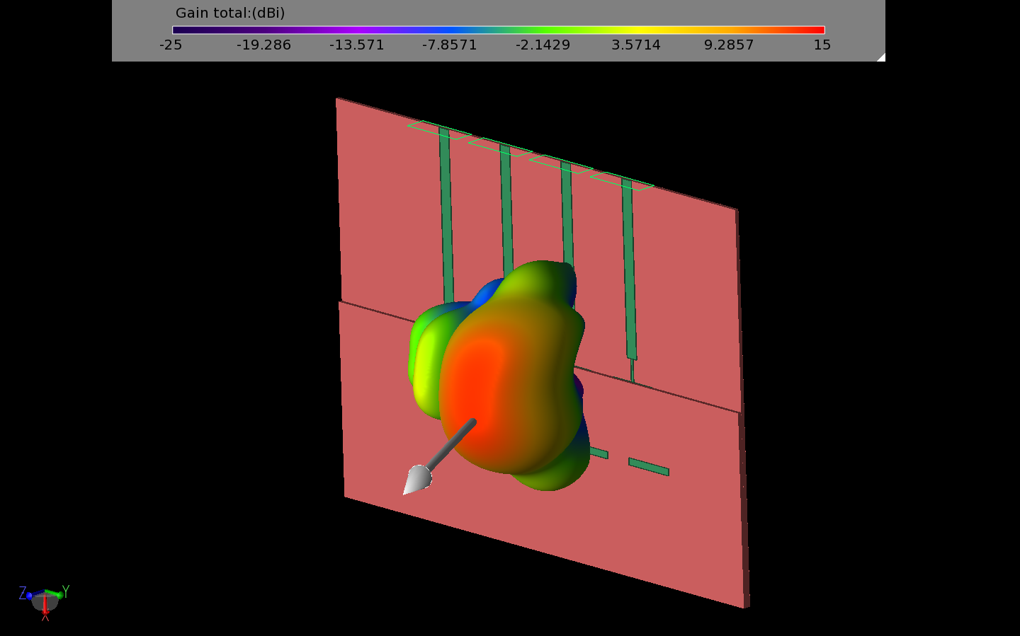
Figure 6: With a phase shift of 90 degrees between the antenna elements the beam shifts about 30 degrees to the side.
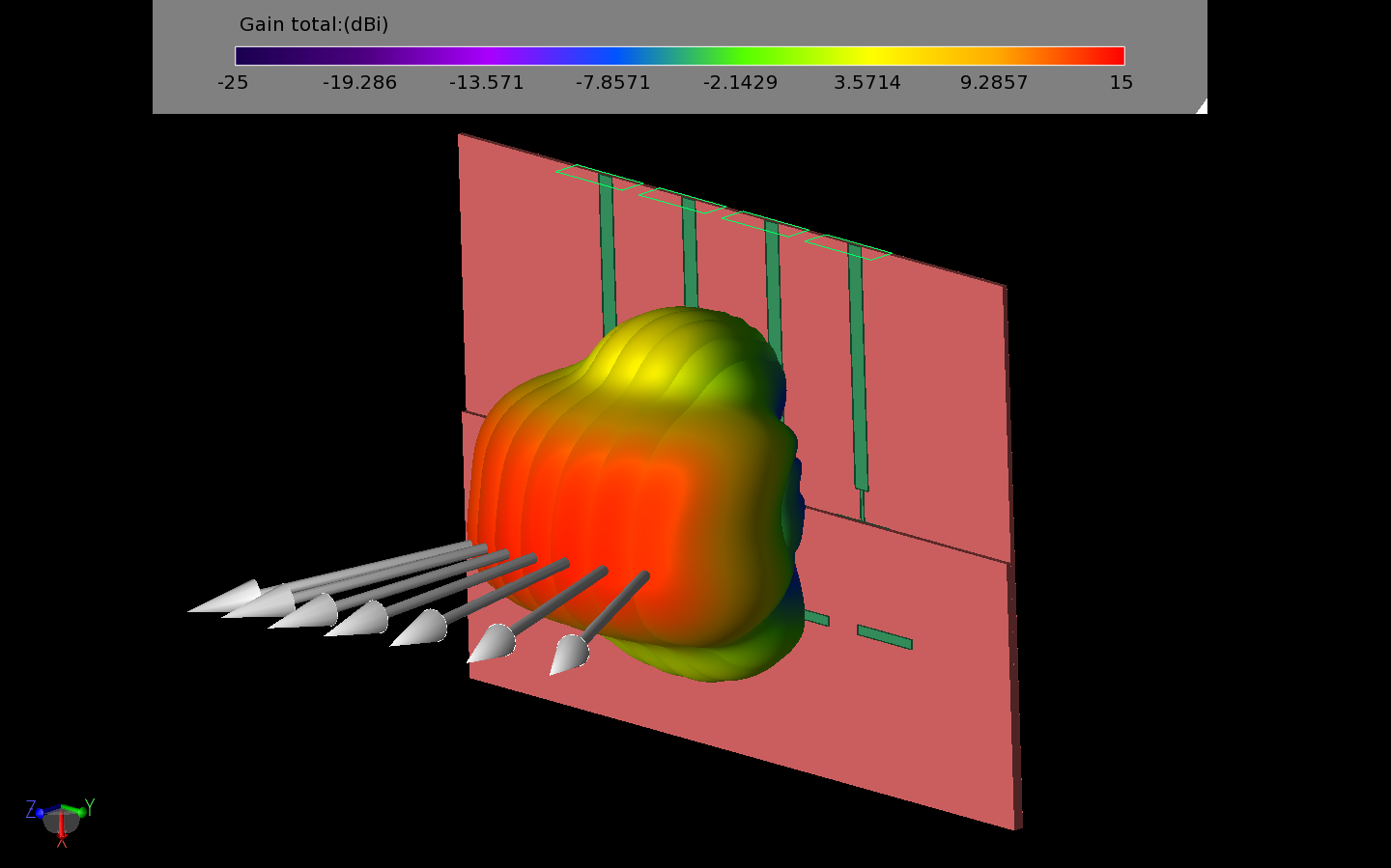
Figure 7: Sweeping the phase shift from -90 to 90 degrees in 30 degree increments generates seven beams that cover a broad area.
The antenna array is next mounted on a virtual reality headset on a phantom head to demonstrate a possible application, shown in Figure 8. Due to the very large size of the head at 60 GHz, a portion of the total problem space, shown in Figure 9, is actually simulated for this demonstration. In Figure 10 the primary beam of the array (all elements in phase) is shown compared to the headset and phantom. When a phase shift of 90 degrees is applied between the elements, the beam shifts to one side by about 30 degrees as shown in Figure 11. Figure 12 demonstrates both beams at the same time.
The dissipated power on the surface of the phantom is also of interest in these applications, and it can be computed by XFdtd. In Figure 13, the dissipated power from the headset-mounted array on the evaluated surface of the phantom model is shown.
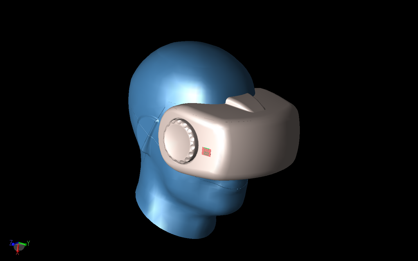
Figure 8: The antenna array is shown mounted on a virtual reality headset. The headset is attached to a phantom head model.
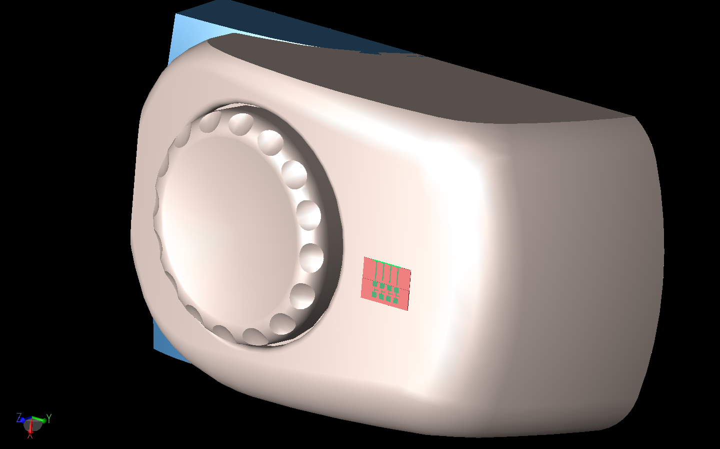
Figure 9: Due to the large size of the problem space, a section of the headset/head model is used for the actual simulations.
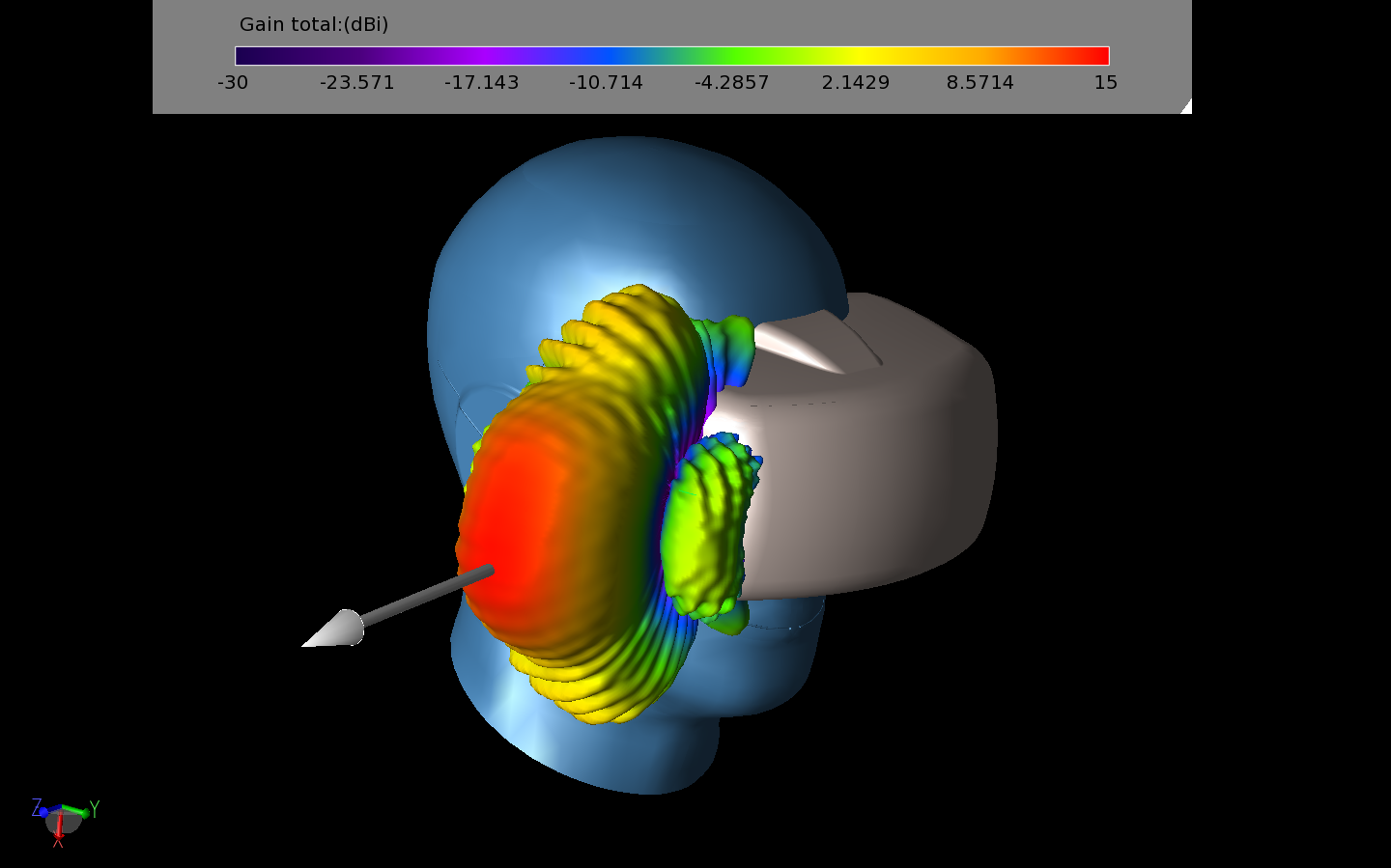
Figure 10: The computed gain pattern for the case of all elements in phase is shown with a strong gain of nearly 15 dBi and a fan-shaped beam.
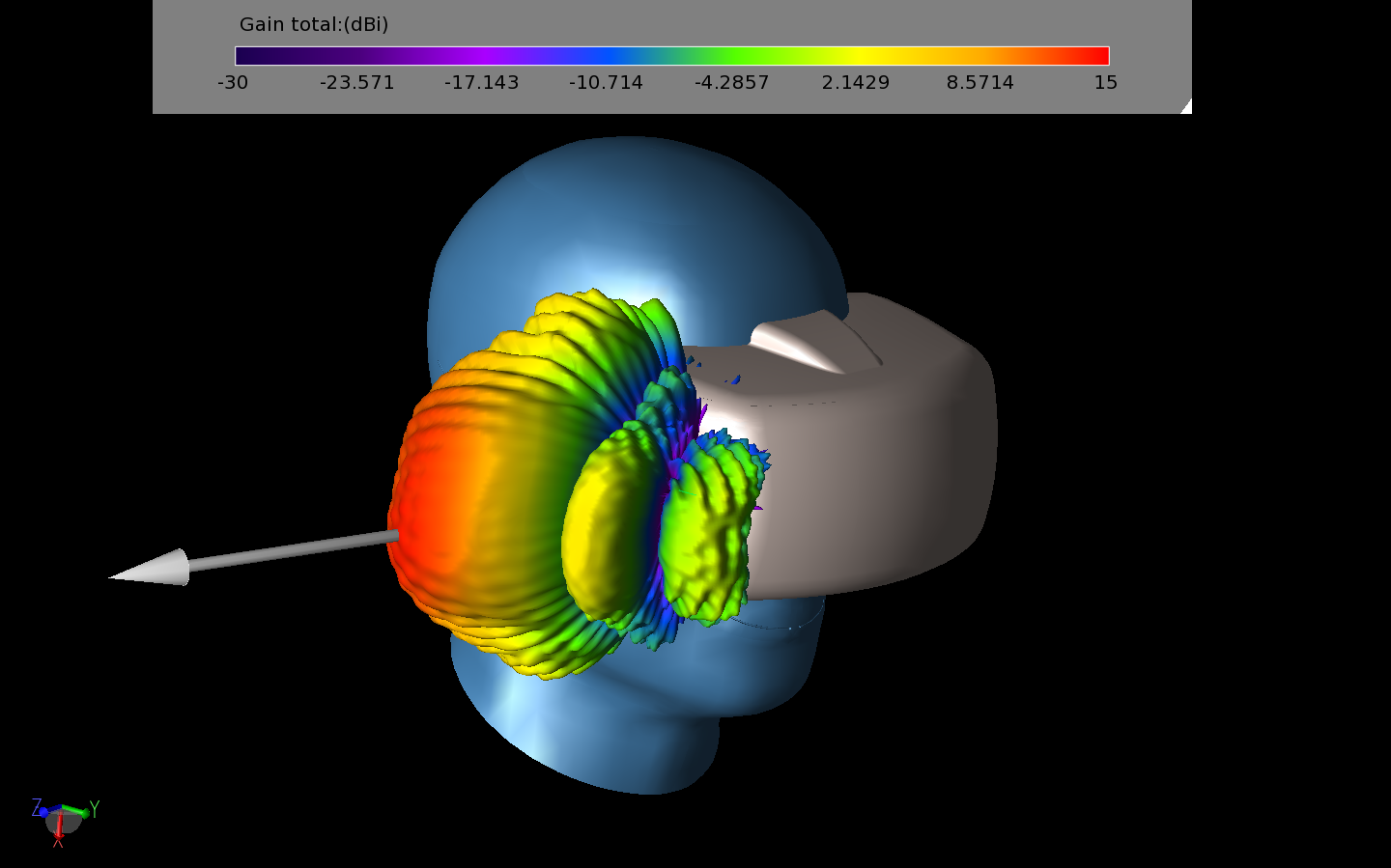
Figure 11: After applying a 90-degree phase shift between the elements the beam is shifted about 30 degrees to the side.
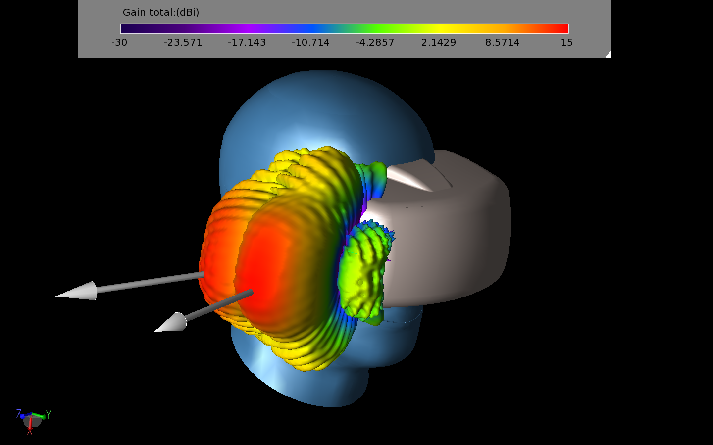
Figure 12: Both beams with 0- and 90-degree phase shifts are shown in this image.
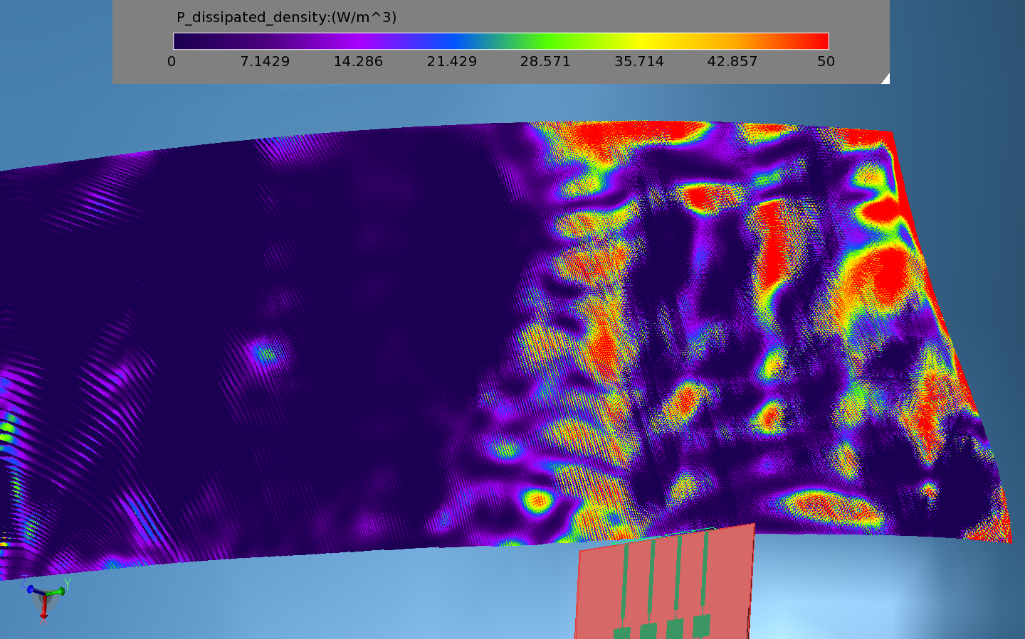
Figure 13: The dissipated power on the surface of the head phantom from the radiating array is computed by the software and displayed.
Reference:
[1] Y. Hong and J. Choi, “60 GHz Array Antenna for mm-Wave 5G Wearable Applications,” 2018 IEEE International Symposium on Antennas and Propagation and USNC/URSI National Radio Science Meeting, pp. 1207-1208, 2018.


