This example serves as a validation exercise for the XFdtd computations of SAR and impedance and was originally performed by Ericsson Radio Systems personnel in the late 1990’s using a much earlier version of the software [1]. The process is repeated here with XFdtd with some modifications including the use of XACT Accurate Cell Technology® meshing on the dipole.
The geometry consists of a liquid-filled spherical bowl exposed to radiation from a dipole antenna placed directly underneath the bowl and offset to one side of the bowl. The configuration at a centered dipole separation (parameter “h”) of 5 mm is shown in Figure 1. The simulations are performed at 835 MHz and the separation distance of the dipole from the bowl is increased from 5 mm to 50 mm and the impact on the SAR and impedance is observed. A secondary position with the dipole offset so that one end of the dipole is directly under the bowl is also simulated and is shown in Figure 2
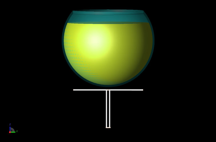
Figure 1: A CAD rendering of the geometry with the dipole centered and the separation distance set at 5mm.
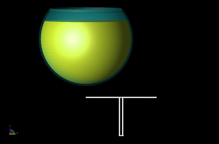
Figure 2: A CAD rendering of the geometry with the dipole offset to the right and the separation distance set at 25 mm.
The antenna is meshed using the XACT feature which exactly conforms to the shape of the geometry. A detailed view of the feed of the antenna is shown in Figure 3 where the source excitation between the dipole arms is highlighted. The base mesh size of the geometry is at 2.5 mm which matches the size used in the reference. In this example the mesh is adjusted to force a cell to be positioned directly over the center of the bowl for more accurately recording the SAR. This mesh adjustment positions the feed of the dipole to be slightly off-center and impacts the impedance results slightly. Note that in the original paper the balun was not included in the simulations but is included in this example. A cross-sectional view of the mesh is shown in Figure 4.
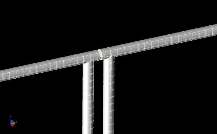
Figure 3: A detailed view of the feed region of the dipole in the XACT mesh.
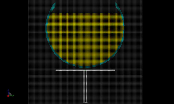
Figure 4: A cross-sectional view of the mesh.
An 835 MHz sinusoidal signal is applied between the dipole arms and the simulation is conducted until steady state is reached with a variation in field energy less than -40 dB down from the peak level. The simulation is performed on an NVIDIA C1060 Tesla GPU card and each dipole position takes about one minute and depends on the separation distance of the dipole from the bowl. Note the original simulations performed in the referenced paper took over five hours with state of the art equipment of the 1990s.
Following the simulation the input power to the dipole is adjusted so that 1 watt of power is delivered to the antenna for all results. The resulting SAR through the cross section of the bowl is shown in Figure 5 for the case of the dipole centered and 5 mm from the bottom of the bowl. Line plots of the SAR originating at the base at the center of the bowl and extending toward the surface of the liquid are compared to measured results and show good agreement. In Figure 6 the SAR versus distance is plotted for three dipole separations with the antenna centered under the bowl.
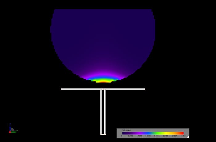
Figure 5: The SAR through the cross section of the sphere with the dipole centered and the separation distance set at 5 mm.
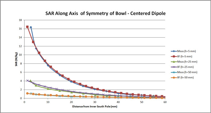
Figure 6: A comparison of the measured and simulated SAR results as a function of distance along the center line of the sphere for three separation distances of the dipole.
The SAR is plotted in horizontal planes at 30 mm and 50 mm above the base of the bowl for the centered dipole case. This is shown in Figures 7 and 8 where the distribution and SAR levels are in good agreement with the measured data in the report.
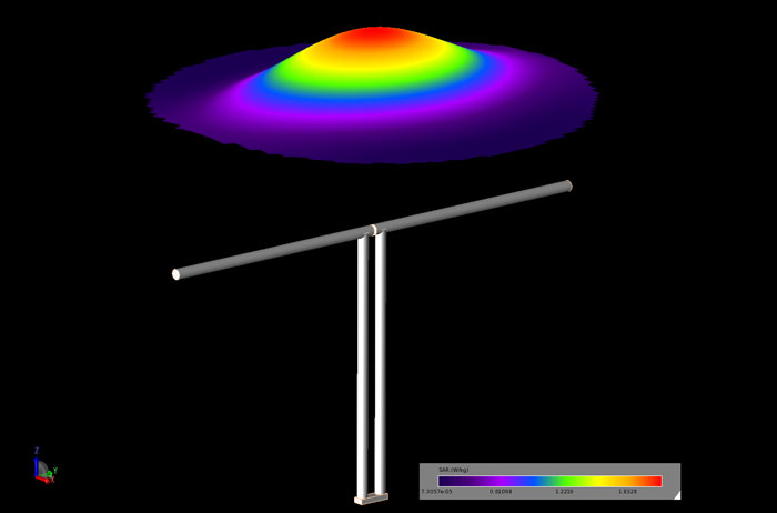
Figure 7: The SAR in a horizontal plane at a distance of 30 mm above the base of the bowl for the centered dipole at a separation distance of 5 mm.
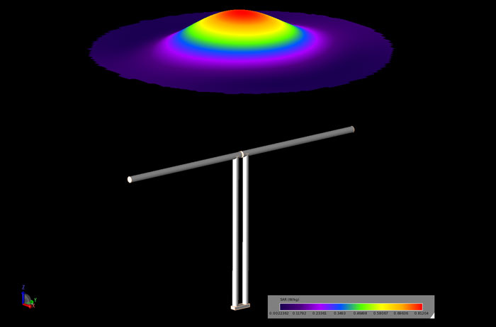
Figure 8: The SAR in a horizontal plane at a distance of 50 mm above the base of the bowl for the centered dipole at a separation distance of 5 mm.
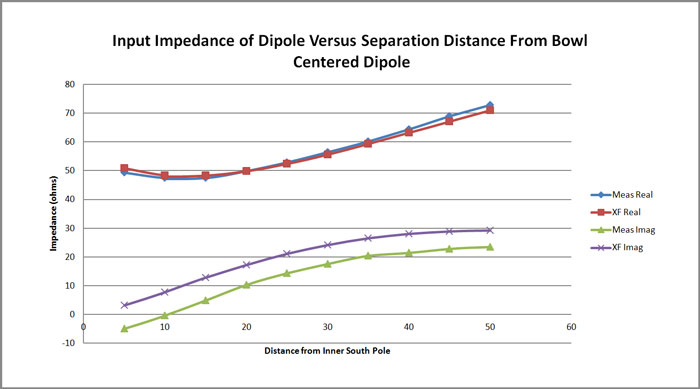
The impedance is also sampled for the different dipole positions. Table 1 shows the dipole impedance compared to the measured values for seven different test positions. In Figure 9 the impedance is plotted for the centered dipole as a function of the separation distance from the bottom of the bowl. The comparison to the measured data is good.
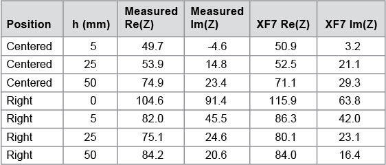
Table 1: A comparison of the measured and simulated impedances for the dipole at several positions relative to the bowl. The parameter h represents the separation distance from the bottom of the bowl. The centered position has the feed point of the dipole centered under the bowl while the right position has one end of the dipole directly under the center of the bowl