In-flight WiFi access is a feature being introduced to many commercials flights to increase customer satisfaction. However, due to the complex cabin environment with varying passenger sizes and seating layouts, it's possible for poor signal reception to occur. Recently a study was performed experimentally where sacks of potatoes were used to simulate passengers in an aircraft in an attempt to eliminate low-signal areas. Simulating such problems on computers with full wave methods was virtually impossible in the past due to the large size of the aircraft cabin and the high frequencies involved. XFdtd makes these simulations possible due to the large memory feature that allows very large calculations requiring over 60 GB of memory, and the new MPI+GPU processing feature that links multiple high-performance graphical processing units in separate computers together through a Message Passing Interface.
In this example the interior of a commercial airliner is used to demonstrate the capability of XFdtd as a platform for optimizing the location of WiFi antennas intended to transmit and receive data from each seat location. This example is intended merely to demonstrate the concept and no specific WiFi system or aircraft configuration is implied. Due to the large size of the aircraft interior and the high frequency of the WiFi system, this simulation is well-suited for the large memory capabilities of XF.
The aircraft section is shown as a CAD model in Figure 1 with the exterior skin of the aircraft not displayed for clarity. The cabin is presumed to be entirely enclosed within a conducting box, so no signal is allowed to radiate outside the aircraft. In Figure 2 drawing of the ceiling, walls, and windows of the CAD model are also disabled so the interior seating arrangement of the aircraft can be seen. The aircraft model is approximately 4.7 x 25.5 x 2.8 meters in size which represents a cubical volume of just under 200,000 wavelengths. The WiFi antennas are considered as simple dipoles and chosen to be located at two positions near the ceiling of the aircraft; one in the forward part of the cabin and one to the rear. Receiver locations are placed in a 3 x 3 grid of dipoles at the seat back location of every other row of the plane as shown in Figure 3. To simplify the addition of these sensors, 405 in total, a script was written and executed. Data stored in this simulation includes the 405 port locations and several planes of the steady-state electric field magnitudes at critical areas of the cabin.
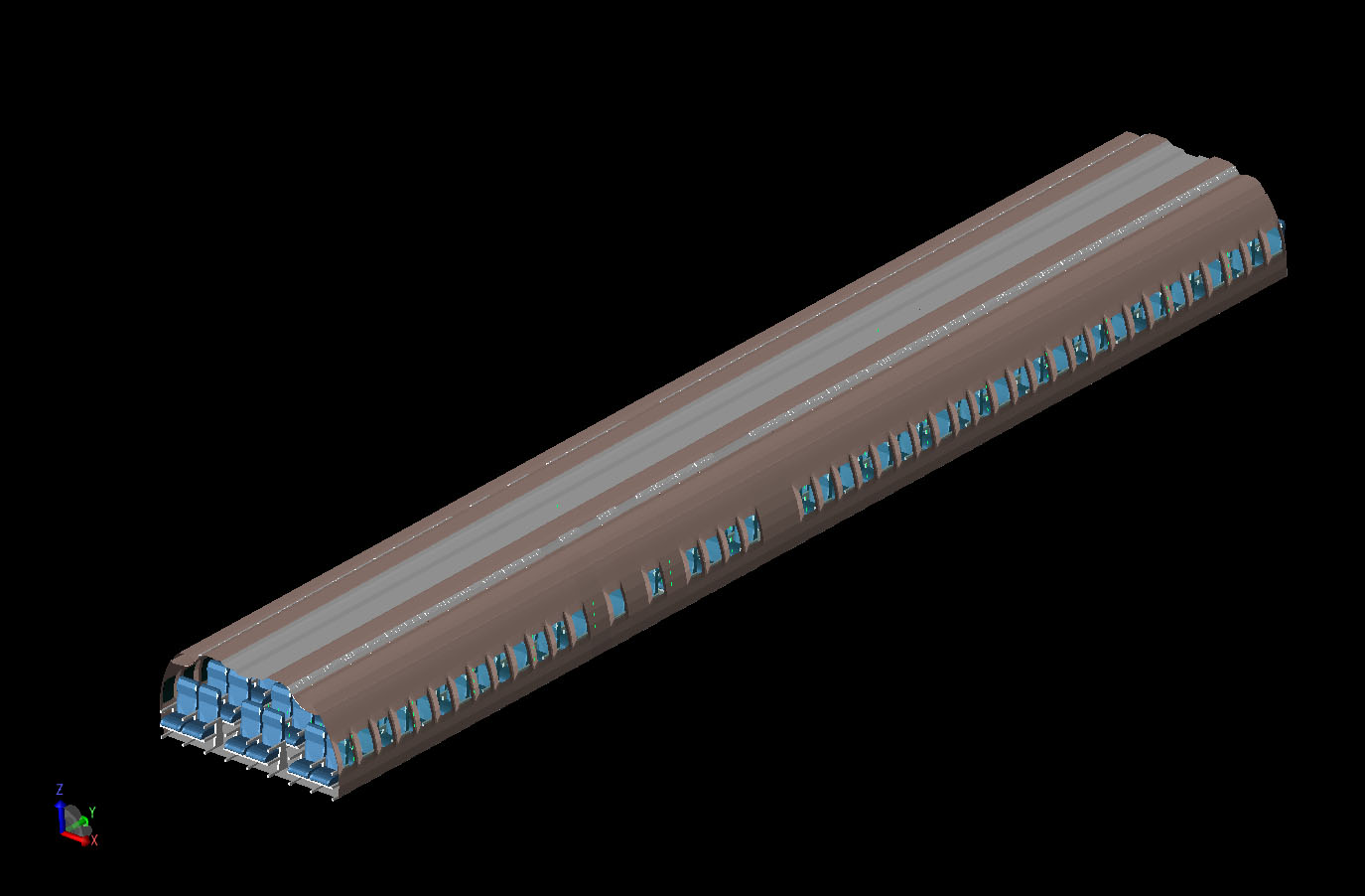
Figure 1: Three-dimensional CAD view of the aircraft cabin with some exterior surfaces removed.
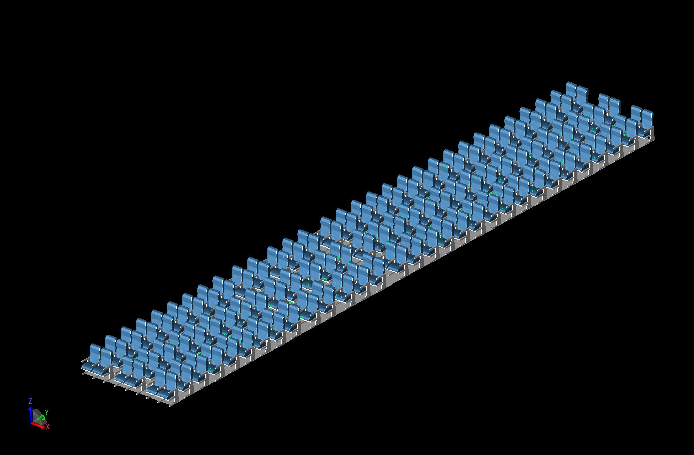
Figure 2: CAD view of the aircraft cabin after the ceilings, walls, windows, and luggage compartments have been removed.
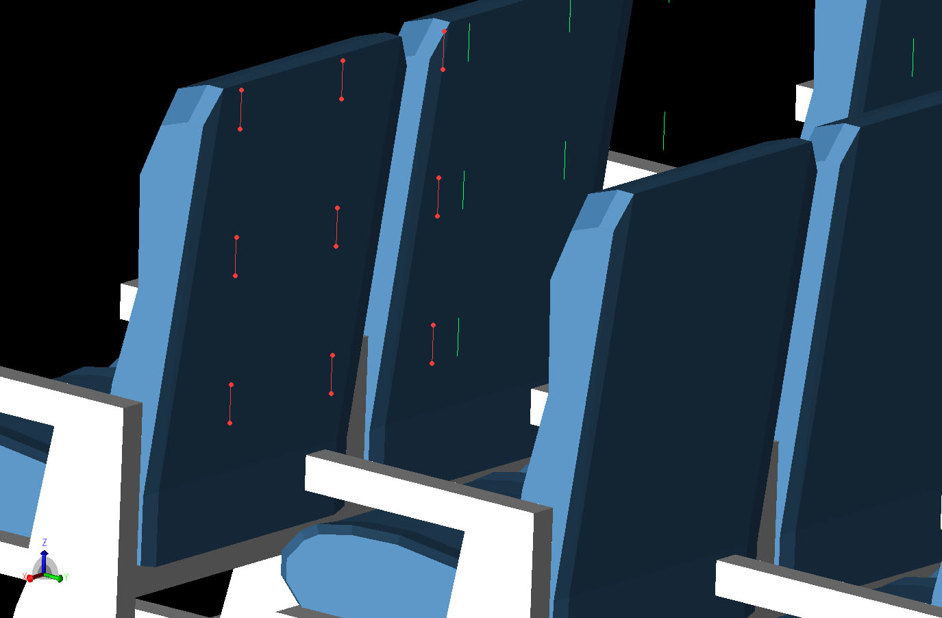
Figure 3: The 3x3 grid of sensor locations defined as dipoles is shown behind one of the seat back locations. The sensor grids are located behind the seats in every other row of the cabin for the first three columns of seats.
The first simulation is with an empty cabin containing only the seats, luggage compartments and other internal features of the aircraft. The simulation provides a baseline for the field propagation throughout the aircraft and will be used to gauge the impact of adding passengers to the seats. In the second simulation, a large male passenger created using Remcom’s VariPose software product is placed in each seat in the aircraft. The passenger is positioned in a seated posture with the arms extended as if hovering over a laptop computer located on the tray table of the seat. A close-up view of a passenger is shown in Figure 4 while a view of the entire filled cabin is shown in Figure 5. In Figure 6 a side view of the cabin is shown with the two transmitter locations near the ceiling and the receiver locations in the seat backs shown in red. Sensor data was saved only for the left side of the aircraft due to symmetry.
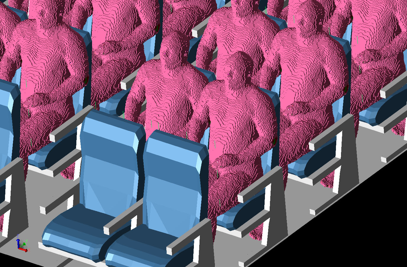
Figure 4: Three-dimensional view of the aircraft cabin with some of the positioned VariPose men in the seats. All seats in the aircraft except the first and last rows have the men seated in them.
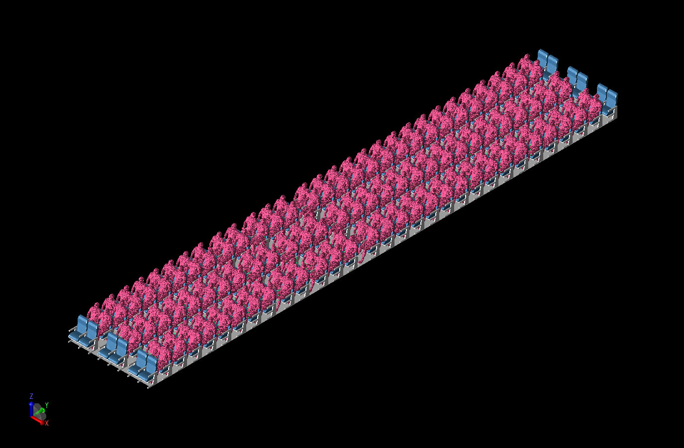
Figure 5: Overall view of the cabin with the men positioned in the seats.
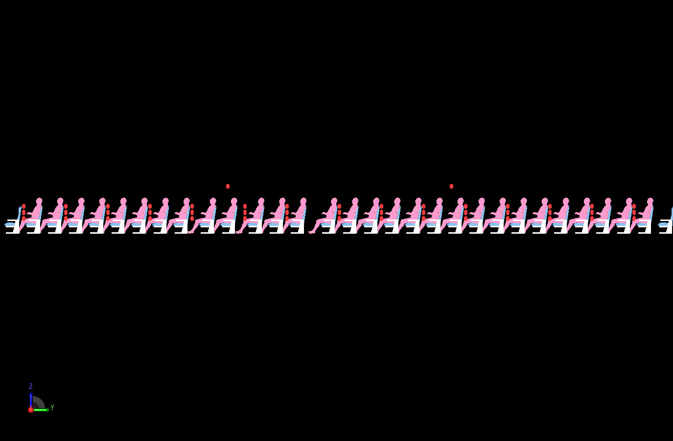
Figure 6: In this side view, the men are shown positioned in the seats and the sensor arrays used for collecting the S-parameter data are shown as red ovals. The two transmitting antennas are at the ceiling level.
The simulations are performed at 2.5 GHz using an FDTD mesh size of 5 mm cubes. Due to the large size of the aircraft cabin, these simulations require 94 GB of memory and contained about 2.84 billion unknowns. They were performed using the MPI+GPU feature of XFdtd on 24 NVIDIA M2090 GPU cards located in the NVIDIA PSG Cluster provided courtesy of the NVIDIA Corporation. Each simulation was run for 30,000 time iterations and took approximately 1 hour, 43 minutes.
Following the simulations, the steady state electric field distribution through several sample planes in the cabin are available for viewing. In Figure 7, the electric field magnitudes through the center of the aisle seat (vertically) and through the headrest (horizontally) are shown for the empty aircraft. The color scale goes from a peak value shown in red at 0 dB down to -70 dB shown in black. The fields in the empty cabin give signal level in the 0 to -30 dB range for much of the space. In Figure 8, the same planes from Figure 7 are shown for the aircraft cabin with the men in the seats. Here the field levels are reduced and there are locations where the field is dropping below -50 dB down from the peak.
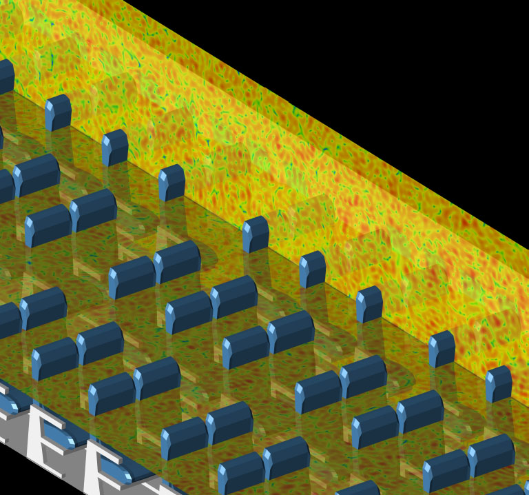
Figure 7: This figure shows the steady-state electric field magnitudes in the cabin when the front transmitter is active at 2.5 GHz. The fields shown are in the plane of the center of the aisle seat vertically and through the center of the 3x3 sensor grid horizontally. The fields show signal strength in the 0 to -30 dB level down from the peak.
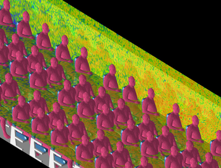
Figure 8: This figure shows the same planar steady-state field locations as Figure 7, but here for the cabin with the men in the seats. Here the field levels are lower in the -50 to -10 dB range down from the peak.
The S-parameter SN,1 for the sample locations is also computed. In this case, the locations selected for the plot shown in Figure 9 are in the center sample point of the 3x3 grid for each row from front to back in the cabin. The plots show the transmission levels for the empty aircraft are relatively flat with variation mainly around -40 dB. In contrast, the full airplane with passengers in the seats shown in Figure 10 shows greater variation in the signal levels with a definite drop in signal toward the back of the cabin.
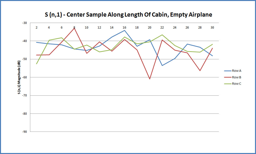
Figure 9: This plot shows the transmitted S-parameter SN,1 for the sensor location in the center of the 3x3 sampling grid as a function of the row in the plane from front to back for the empty aircraft.
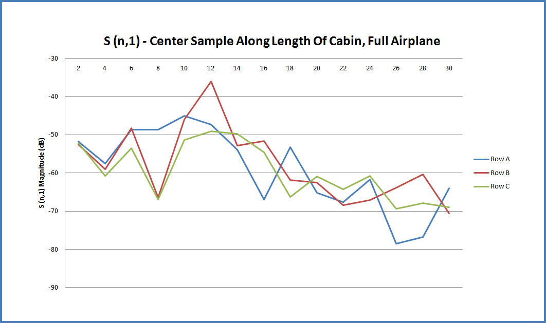
Figure 10: This plot shows the transmitted S-parameter SN,1 for the sensor location in the center of the 3x3 sampling grid as a function of the row in the plane from front to back with the seats occupied by the men.
The simulations shown here could be expanded greatly by introducing better antenna models, other frequencies, different seating configurations and more. This example merely presents one possible simulation that is made possible by the large memory and fast processing capabilities in XFdtd.