A variation on a Luneburg lens is formed by creating two concentric dielectric spheres. The inner sphere has a relative permittivity of 1.7 and a radius of 125 mm while the outer sphere has a relative permittivity of 1.4 and a radius of 250 mm. A 600 x 600 x 10 mm dielectric slab of relative permittivity 2 is placed 100 mm behind the sphere to represent the surface of a plastic box enclosing the lens. The completed structure, displayed in Figure 1, is illuminated with a vertically polarized 15 GHz plane wave traveling along the y-axis originating on the opposite side of the lens from the dielectric slab. Figure 2 shows a cross section of the completed geometry. Taking the dielectric constants into account, the completed geometry is tens of wavelengths long per side. A structure this electrically large would have once represented a formidable challenge; however, advances in computer technology and the FDTD method have made this a very reasonable simulation today. A modern 4-core workstation running XFdtd can reach the solution in less than two hours.
A uniform base cell size of 1.9 mm is chosen to satisfy the Courant limit in free space, and an automatic grid region of 1.5 mm is placed on the outer sphere. This grid region will yield more than 10 cells per wavelength within the denser sphere materials. Absorbing PML boundaries are used on all sides with 10 cells of free space padding in the +/-x, +/-z, and -y directions. The +y direction is given 30 cells of free space padding. The resulting mesh occupies 76.4 million cells and requires 3.2 GB of RAM to simulate.
The movie displays an animated sequence of electric fields versus time. The movie begins by slicing through the geometry to the center of the sphere to help give a point of reference. The geometry is then hidden in order to make it possible to view the fields within the lens. A discontinuity in the fields is visible around the boundary of the animation. This is an artifact of the total field/scattered field simulation technique used in this example. Total field/scattered field simulations use a hybrid approach to simultaneously calculate scattered field values near the simulation boundary and total field values over the rest of the simulation space, and the visible field discontinuities are the scattered field portions of the computation. The movie clearly demonstrates the focusing effect of this structure.
Figure 3 shows the steady-state E field magnitudes through the center of the lens and on the top surface of the plastic slab.
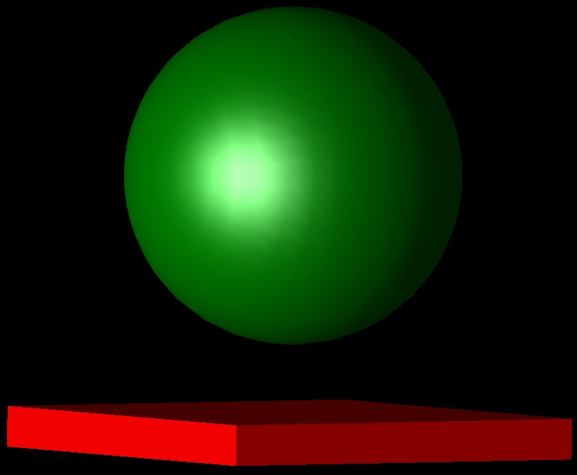
Figure 1: Completed solid geometry
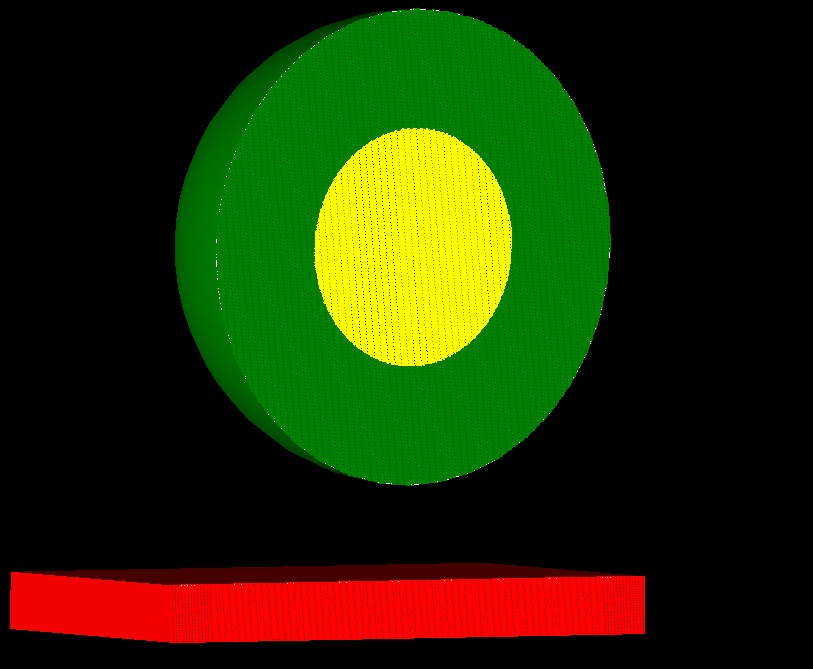
Figure 2: Cross section of geometry with mesh

Figure 3: Steady-state electric field magnitudes