To demonstrate some of the capabilities of Wireless InSite to make indoor propagation predictions, it is applied to the first example in the paper "A Ray-Tracing Method for Modeling Indoor Wave Propagation and Penetration" by Yang, Wu, and Ko, IEEE Transactions on Antennas and Propagation, June 1998. The geometry and wall material information is given in Figure 1. There are no dimensions given for the wall spacing and thickness, so these must be estimated from the figure.
Figure 1
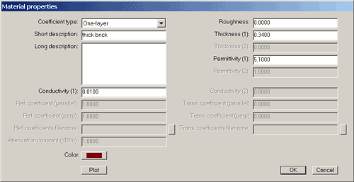
Figure 2
To start the Wireless InSite calculation, we start WI and begin a new project from Project>New>Project. Next we add a floor plan as Project>New>Feature>Floor Plan. With a floor height of 0 meters and ceiling height of 3 meters the floor plan editor window opens. We first define the necessary wall types in Wireless InSite from the information in Figure 1, using different colors to differentiate the wall materials. The specification for thick Reinforced Concrete wall is shown in Figure 2.
This window is obtained by right-clicking on the appropriate entry in the project hierarchy (see Figure 3).
After defining the wall materials and thickness the floor plan editor window is used to draw the walls. The floor and ceiling is also added using this editor. The result is shown in Figure 4.
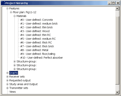
Figure 3
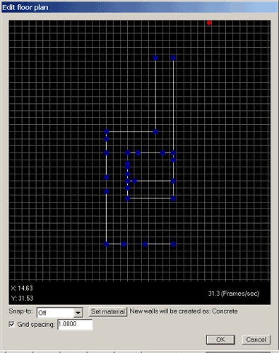
Figure 4
The next step is to add the transmitter and receiver (antenna) locations. Before making the calculation for the transmitter/receiver sets shown in Figure 1, we first want to calibrate the transmitter power as described in the paper. This calibration involves placing the transmitting and receiving antennas 1 m apart and 1.3 m above the floor in the open area of hallway. We locate these antennas in a similar fashion as the walls using editor windows that open from Project>New>Transmitter Set>Points and Project>New>Receiver Set>Points. The geometry with transmitter and receiver located for the calibration calculation is shown in Figure 5.
The ceiling is set to "invisible" so that the walls and floor can be seen. In order to make the calculations we specify vertical linear dipole antennas, a narrowband waveform with a frequency of 900 MHz, and a study area. These all correspond to the tabs at the top of the Wireless InSite Main Window as shown in Figure 6.
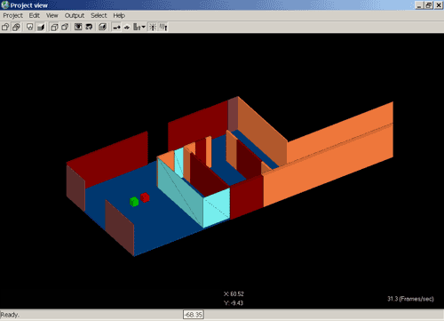
Figure 5
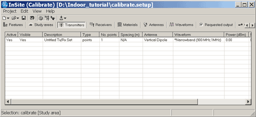
Figure 6
The Study Area is manually drawn to completely enclose the entire floor plan. The calculation is done with the 3D ray-shooting model with 4 wall transmissions, 2 wall reflections and fully correlated. Properties of the other parameters of the calculation are all available from the Wireless InSite main window by selecting the appropriate tab and right-clicking on the item.
After saving all files with an appropriate file name, we are ready to make the calibration calculations from Project>Run>New. After a couple of seconds this is completed. The power at the receiver is obtained by clicking down the project hierarchy tree "Study Areas and Output">"Point-to-Multipoint">"Transmitter#1-Receiver#1". A right-click on this entry and choice of "properties" shows a received power of -29.66 dBm. Since this is the 0 dB calibration point for the results given in the paper, and since it was obtained by Wireless InSite for a transmitter power of 0 dBm (the default), for the remaining calculations we set the transmitter power to +29.66 dBm (right-click on the transmitter entry in the main window and then click on properties) so that this calibration calculation, if repeated, would show a received power of 0 dBm. The rays propagating from the transmitting to receiving antenna for the calibration calculation are shown in Figure 7.
We are now ready to make calculations for the transmitter and receiver locations shown in Figure 1. To do this we first delete the transmitter and receiver locations used for calibration, and then add a new transmitter location and a pair of receiver routes. The receiver spacing and collection area are made smaller than the default values since the distances for this simple example are so short. The heights are adjusted from the "edit control points" window that opens from the Tx/Rx properties window shown in Figure 8.
The result is shown in Figure 9.
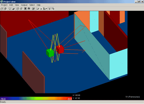
Figure 7
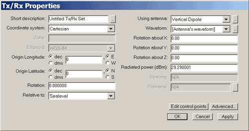
Figure 8
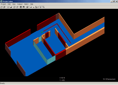
Figure 9
In figures 11 and 12 of the paper measured results are given for the transmitting antenna located at heights of 1.3m in Figure 11 and 1.96m in Figure 12, with the receiver heights always at 1.3m. Measured results for the receivers in Section A are given in figures 11a, 12a of the paper, and for Section B receivers are in figures 11b, 12b. The measured results were manually read from the figures in the paper and written to text files. The text files of measured received power were imported into Wireless InSite for plotting.
Wireless InSite results which include fast fading (retain "all" phase information set in the advanced study area properties) are compared with measured results from the paper in Figures 10-13.
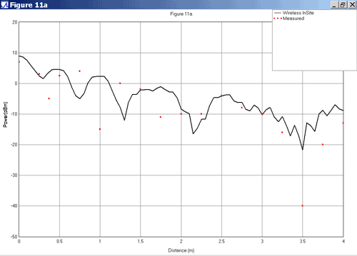
Figure 10
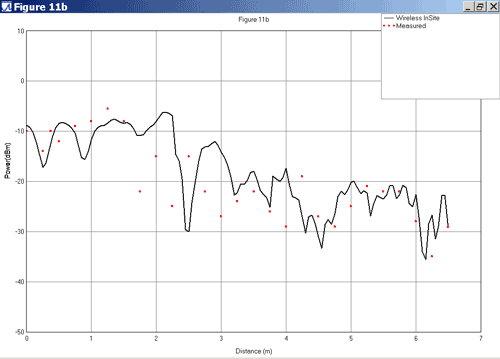
Figure 11
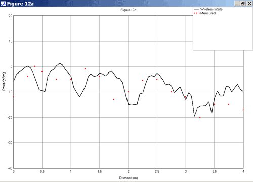
Figure 12
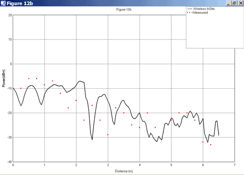
Figure 13
The Wireless InSite results cannot reproduce the fast fades of the measurements since the wall locations and thickness are not specified accurately in the paper. Given this, the agreement is quite good. For comparison, a Wireless InSite calculation in the uncorrelated mode, ignoring the phases of the different rays, is shown in Figure 14.
As expected this result shows the power arriving at the receiving antenna from all rays without including the cancellation due to the rays arriving with different phase and follows the peaks of the measurements. Ray paths for a transmitter-receiver pair are shown in Figure 15.
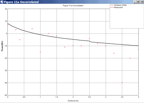
Figure 14
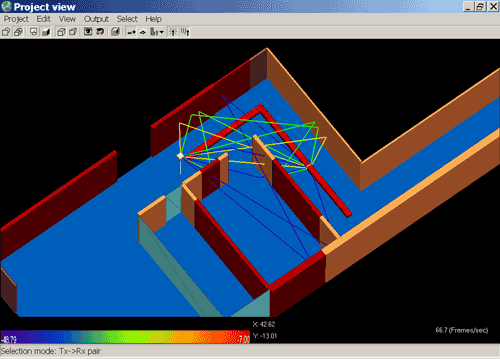
Figure 15
The figures included with this example indicate the ability of Wireless InSite to organize, control, and display all the data needed for a radio propagation calculation. They don't convey the calculation speed of Wireless InSite. In the Yang et all paper tables of computer time are given for their various calculations. Their computer times are typically an hour or longer to obtain results for one transmitter and one of the receiver sections.