The four targets consist of small bodies of revolution that were measured at several frequencies for monostatic RCS around the azimuthal axis. The targets were developed by NASA and published in [1]. The measured results used in this example were extracted from the later publication [2].
The target shapes were chosen to highlight challenging situations for simulation software such as smoothly curved surfaces. The four bodies of revolution simulated here include a symmetrical single ogive, a double ogive, a half-cone, half-sphere shape, and a similar cone sphere shape with a small gap encircling the connection point between the cone and the sphere. The four targets are shown in Figures 1-4.
-
Figure 1 shows the Single Ogive geometry with a total length of 10 inches (254 mm) with a maximum radius of 1 inch (25.4 mm).
-
Figure 2 shows the Double Ogive with a maximum length of 7.5 inches (190.5 mm) and a maximum radius of 1 inch (25.4 mm). The +X side of the Double Ogive matches the Single Ogive structure while the –X side has a larger angle.
-
Figure 3 shows the Cone-Sphere geometry with an overall length of 26.768 inches (679.9072 mm) and the cone section having a length of 23.821 inches (605.0534 mm) with a base of radius of 2.947 inches (74.8538 mm). The radius of the sphere section matches the base of the cone section.
-
Figure 4 shows the Cone-Sphere with Gap geometry, which matches the Cone-Sphere shown in Figure 3, but with a small gap included in the half-sphere section at the intersection with the cone. The gap is 0.25 inch (6.35 mm) wide and deep.
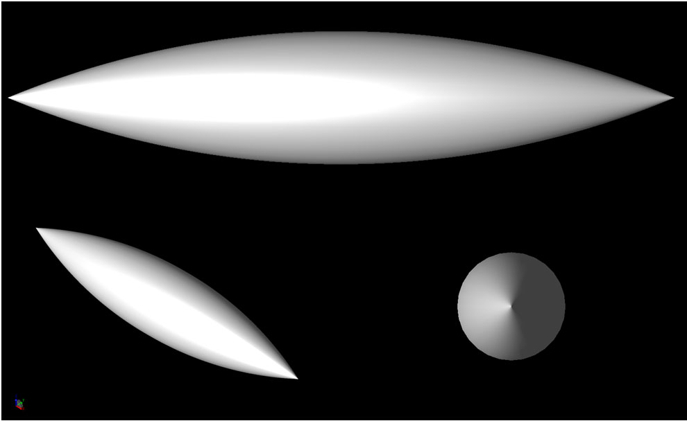
Figure 1: The Single Ogive geometry.
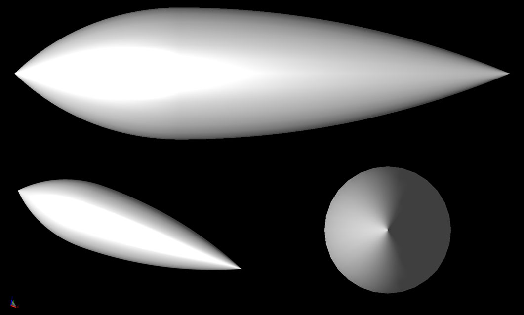
Figure 2: The Double Ogive geometry.
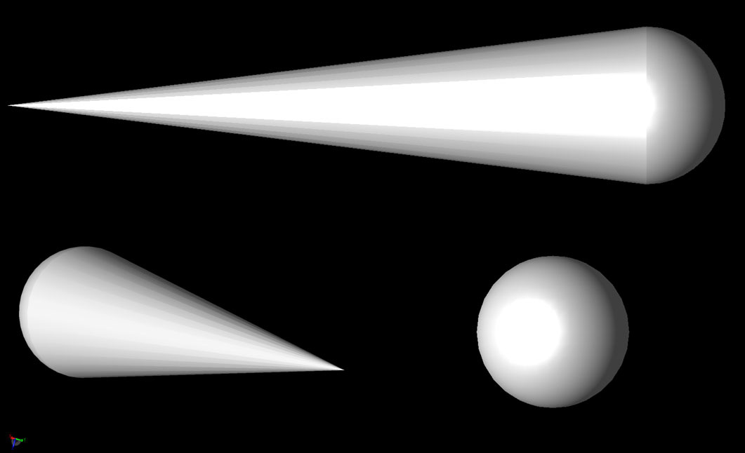
Figure 3: The Cone-Sphere geometry.
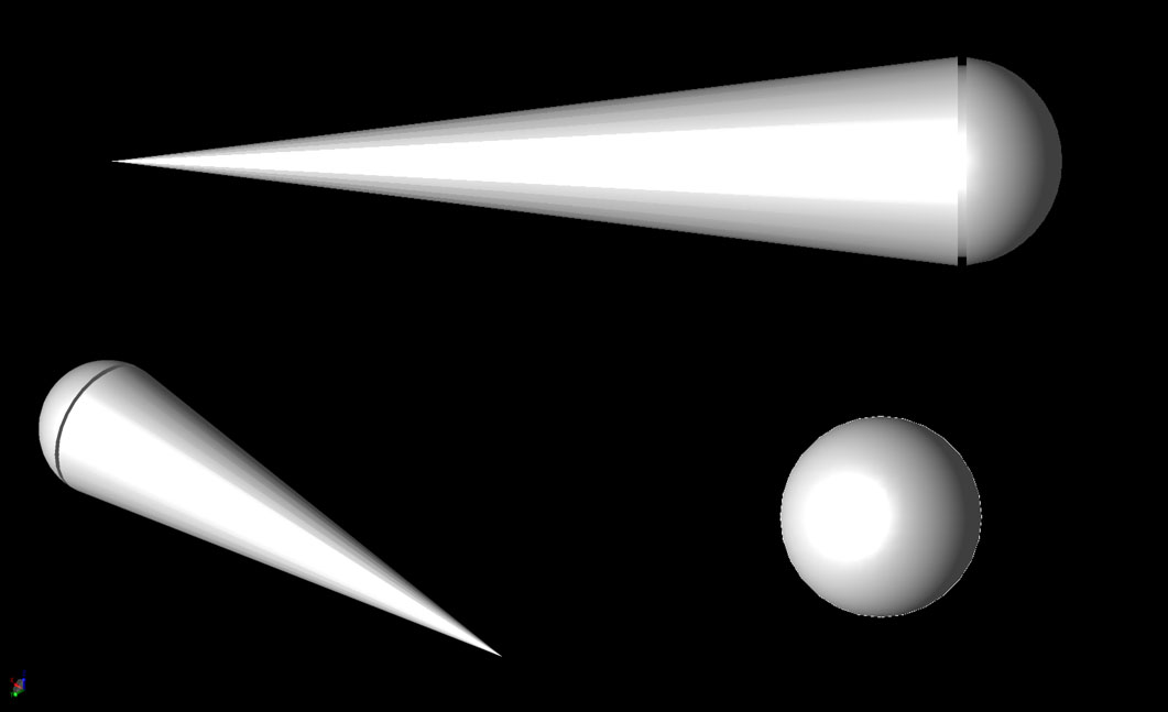
Figure 4: The Cone-Sphere with Gap geometry.
The simulations were performed using XFdtd with the XACT Accurate Cell Technology meshing feature used for all targets. The software used a mesh size equivalent to 20 cells per wavelength at the frequency of the simulation. The fixed points feature was employed for all geometries and manual fixed points were added at the vertices of the ogives and cones. In some cases good results were possible with a lower resolution, but for consistency all results are shown in the same resolution. To better illustrate the fidelity of the simulation, a view of the XACT mesh is shown in Figure 5 for the Single Ogive geometry at 20 cells per wavelength resolution for a frequency of 1.18 GHz.
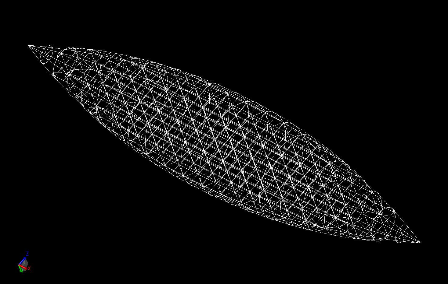
Figure 5: A view of the XACT mesh of the Single Ogive geometry.
The simulations used an incident plane wave with a sinusoidal source and data was collected using a steady-state far zone transform. This combination was shown to give the most rapid results for this single-frequency analysis. Due to the results required in a backscatter RCS situation, each simulation produced a single data point for the file output graph.
The XStream GPU solution was used to perform all simulations to provide the quickest results. A single value parameter sweep was performed with the incident phi direction (azimuth angle) used as the parameter in increments of one degree. The output was processed with a custom script written to extract the backscatter RCS at each incident angle and plot the results in a single graph. The simulation execution times varied with the frequency geometry, but generally required less than 20 seconds per angle for the lower frequencies and less than 5 minutes per angle for the higher frequencies on an NVIDIA Tesla C1060 GPU card.
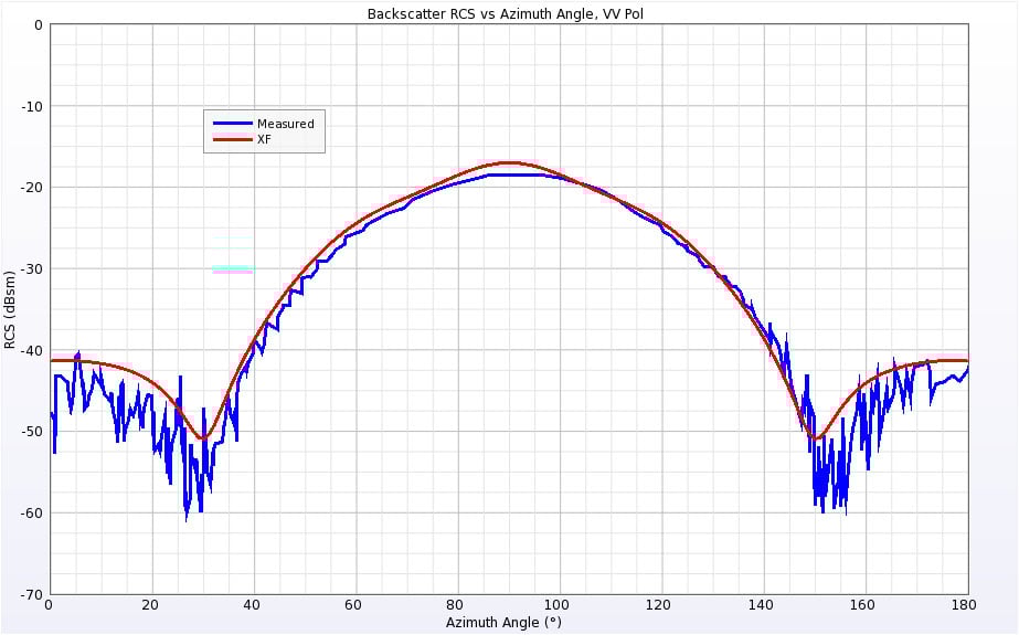
Figure 6: Backscatter RCS for Single Ogive at 1.18 GHz for vertical polarization.
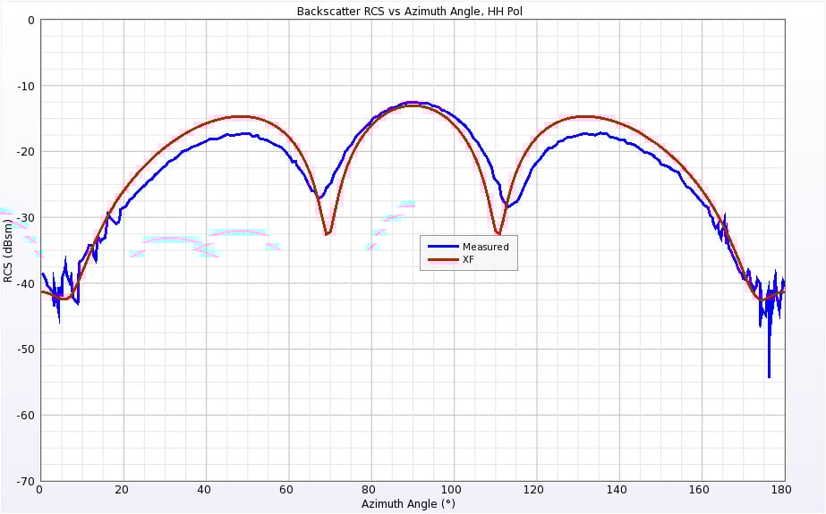
Figure 7: Backscatter RCS for Single Ogive at 1.18 GHz for horizontal polarization.
The Single Ogive geometry is aligned with the X axis, so an incident angle of zero degrees strikes the point of the ogive while an angle of 90 degrees hits the side. The Single Ogive was simulated at two frequencies: 1.18 GHz where the ogive is approximately one wavelength long, and 9 GHz where the ogive is about 8 wavelengths long. The simulated results compared to measured results from the referenced publications at 1.18 GHz are shown in Figures 6 and 7 for the vertical and horizontal polarizations, respectively. The results show generally good agreement over all incident angles. Similarly, the results for 9 GHz are shown in Figures 8 and 9.
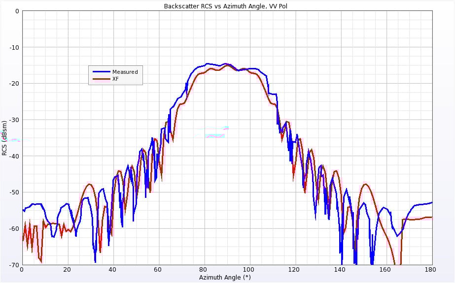
Figure 8: Backscatter RCS for Single Ogive at 9 GHz for vertical polarization.
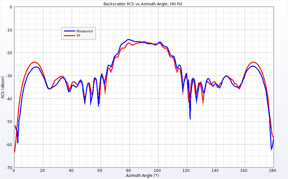
Figure 9: Backscatter RCS for Single Ogive at 9 GHz for horizontal polarization.
The Double Ogive is aligned along the X axis like the Single Ogive. The blunter end of the ogive is towards the –X direction while the end that matches the Single Ogive curvature is pointing in the +X direction. The Double Ogive was simulated at 1.57 GHz and 9 GHz. The RCS results for both frequencies and both polarizations are shown in Figures 10 through 13. The agreement with the measurements is generally good, although there are some points, such as near broadside for the low frequency horizontal polarization, that show several decibels of variation. In the original published work, the author’s simulations showed very similar results to those obtained with XFdtd.
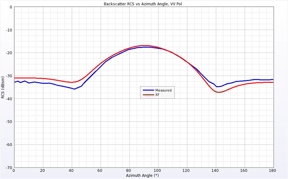
Figure 10: Backscatter RCS of Double Ogive at 1.57 GHz for vertical polarization.
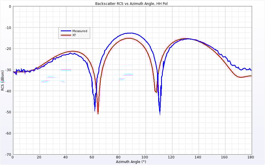
Figure 11: Backscatter RCS of Double Ogive at 1.57 GHz for horizontal polarization.
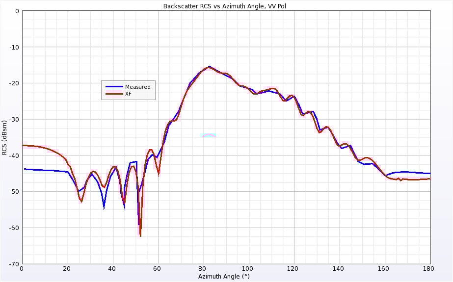
Figure 12: Backscatter RCS of Double Ogive at 9 GHz for vertical polarization.
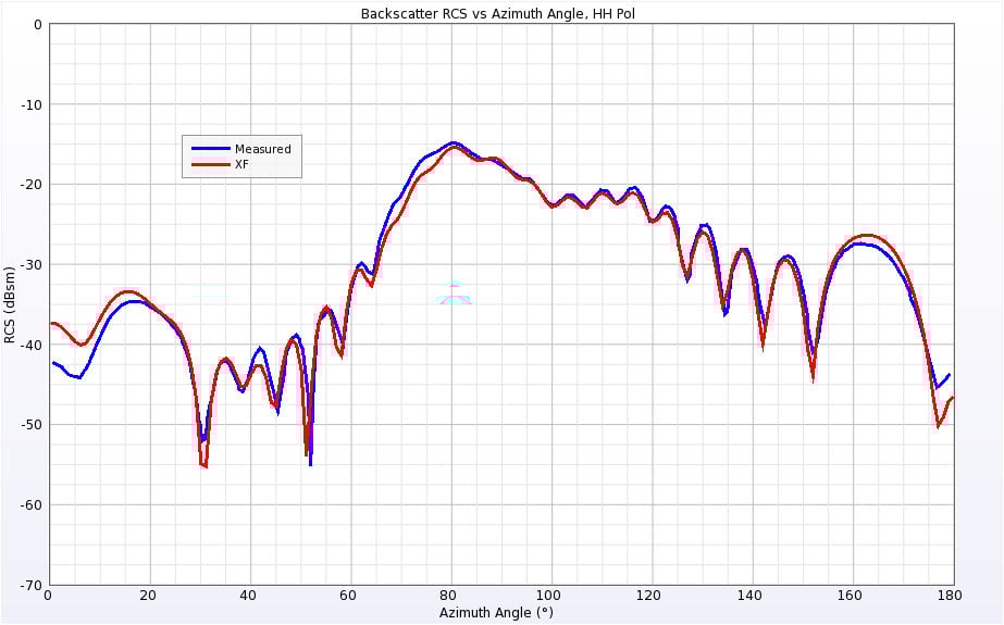
Figure 13: Backscatter RCS of Double Ogive at 9 GHz for horizontal polarization.
The Cone-Sphere geometry lies along the X axis and has a conical point facing in the –X direction and a spherical end in the +X direction. The Cone-Sphere was simulated at 0.869 GHz and 9 GHz. The RCS results for both frequencies and polarizations are shown in Figures 14 through 17. At the lower frequency there is some variation between the simulated and measured results when the incident angle nears the point of the cone. Very similar variation was observed in the published results with the author’s simulations. Also, the geometry is completely symmetrical at 0 and 180 degrees for both polarizations and the XFdtd results match at the end points while the measurements show several decibels of difference, making it seem likely there is some error in the measured results at those angles.
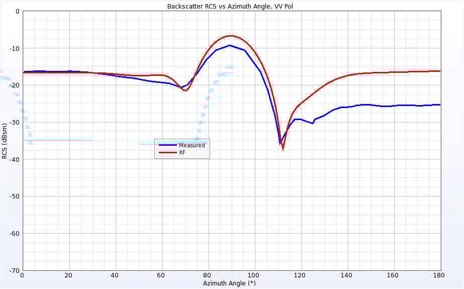
Figure 14: Backscatter RCS of Cone-Sphere at 0.869 GHz for vertical polarization.
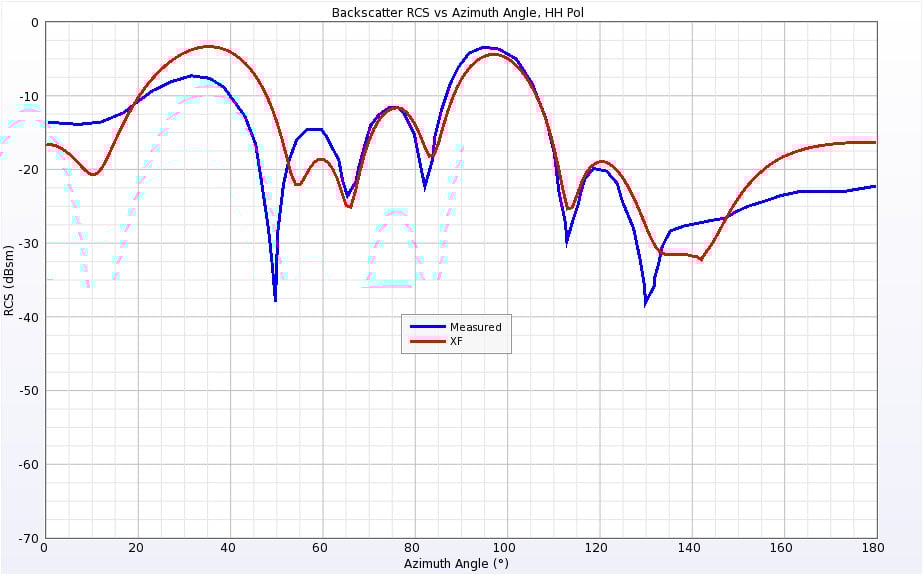
Figure 15: Backscatter RCS of Cone-Sphere at 0.869 GHz for horizontal polarization.
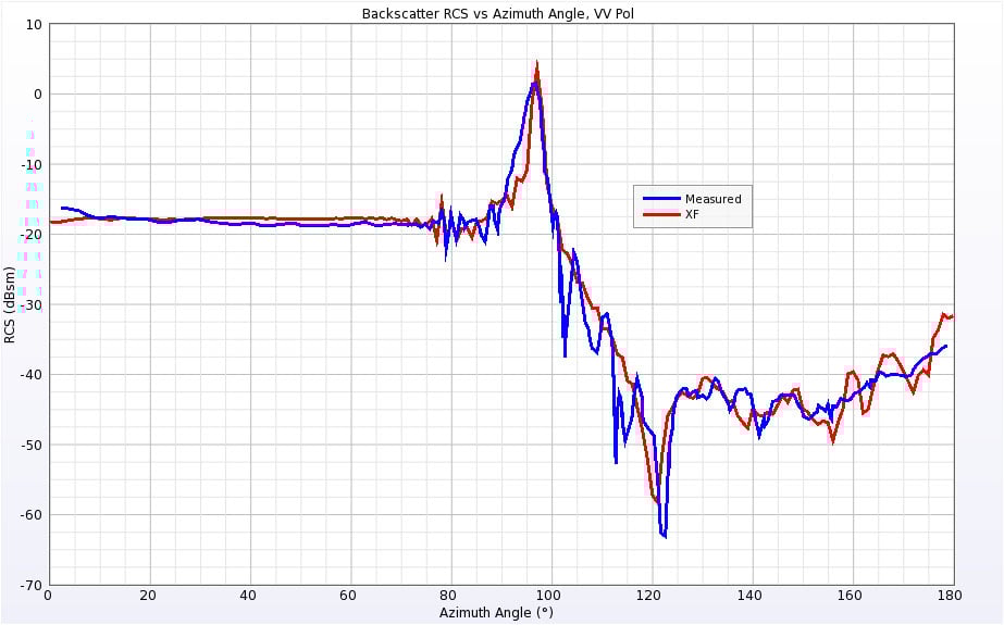
Figure 16: Backscatter RCS of Cone-Sphere at 9 GHz for vertical polarization.
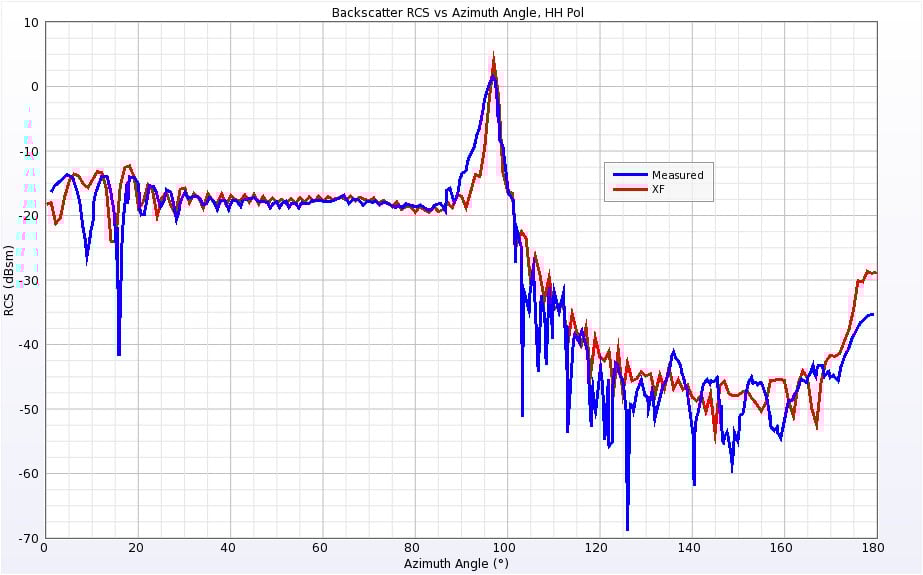
Figure 17: Backscatter RCS of Cone-Sphere at 9 GHz for horizontal polarization.
Finally, the Cone-Sphere with Gap geometry is aligned like the Cone-Sphere geometry. The structure was simulated at the same frequencies of 0.869 GHz and 9 GHz as well. The results are shown in Figures 18 through 21 and have similar characteristics to the Cone-Sphere results.
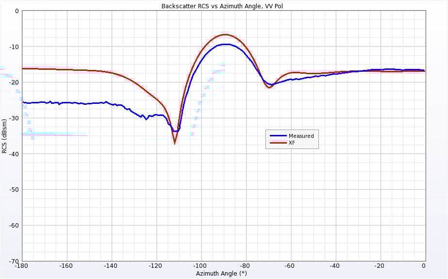
Figure 18: Backscatter RCS of Cone-Sphere with Gap at 0.869 GHz for vertical polarization.
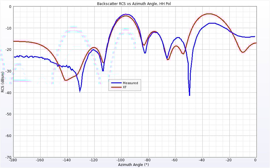
Figure 19: Backscatter RCS of Cone-Sphere with Gap at 0.869 GHz for horizontal polarization.
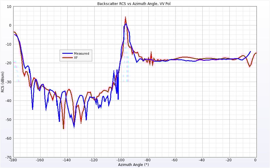
Figure 20: RCS for Cone-Sphere with Gap at 9 GHz for vertical polarization.
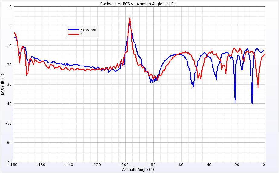
Figure 21: RCS for Cone-Sphere with Gap at 9 GHz for horizontal polarization.
References
-
H. T. G. Wang, M. L. Sanders, A. C. Woo, and M. J. Schuh. “Radar Cross Section Measurement Data, Electromagnetic Code Consortium Benchmark Targets.” NWC TM 6985, May 1991.
-
A. C. Woo, H. T.G. Wang, M. J. Schuh, and M. L. Sanders. “Benchmark Plate Radar Targets for the Validation of Computational Electromagnetics Programs.” IEEE Antennas and Propagation Magazine, vol. 35, no. 1, February 1993.