This Vivaldi antenna design was originally proposed as a benchmark simulation problem by Microwave Engineering Europe magazine in the early 2000s. Here the classic example is updated with TEM ports and an expanded frequency range.
The antenna design is a balanced Vivaldi comprised of three metal layers surrounding a Duroid substrate and it is built entirely within XFdtd using the CAD model generation tools. The top and bottom layers are identical and the feed is applied through the middle layer. The metal portions of the structure are shown in Figures 1 and 2. The geometry is oriented so that the Z axis runs along the long dimension of the antenna while the X axis spans the width. The structure is meshed using the XACT Accurate Cell Technology conformal meshing feature to accurately capture the curvature of the antenna edges. The meshed metal structures at a cell size of 0.5 mm are shown in Figure 3.

Figure 1: CAD view of the Vivaldi outer conductor. An identical part is on the top and bottom of the substrate.
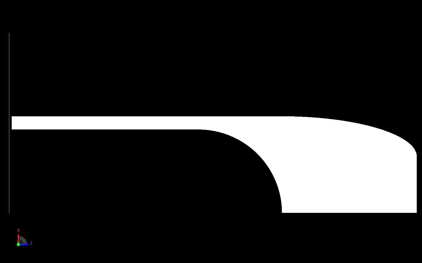
Figure 2: CAD view of the Vivaldi center conductor.
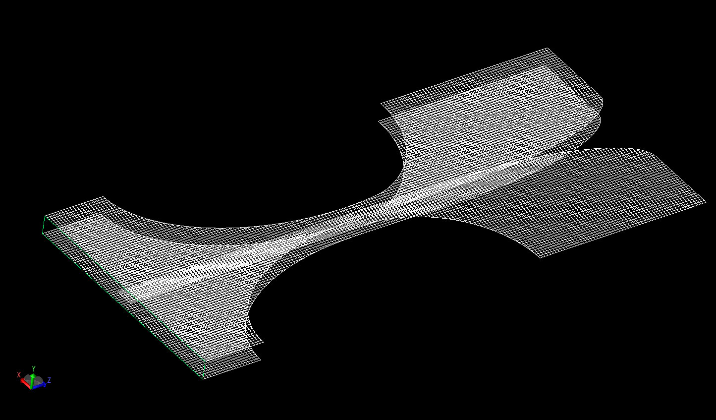
Figure 3: Mesh view of the Vivaldi antenna at a resolution of 0.5 mm.
In previous versions of this example a component feed was added to mimic the SMA launcher used to excite the antenna. Here the waveguide ports of XF are used to create a TEM excitation at the input of the antenna, as shown in Figure 4. This addition allows the simulation to be independent of any effects added by the meshing of the feed structure.
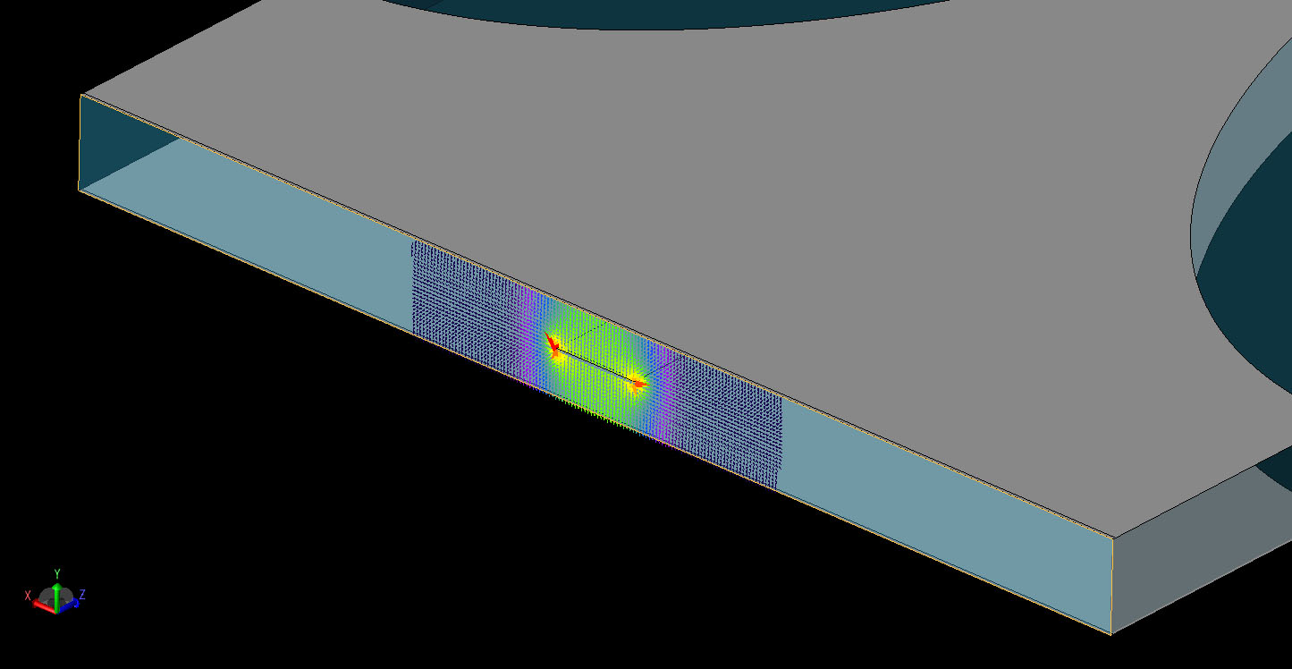
Figure 4: Detailed view of the TEM port excitation used to simulate the antenna.
To determine the best resolution for the simulation, the mesh size is parameterized and several iterations of the design are computed from 0.75 mm down to 0.125 mm. The memory requirements for this sweep range from 75 MB to 1.3 GB and the execution time to a -30 dB convergence level on an NVIDIA Quadro 3000M graphics card vary from 28 seconds to about 18 minutes. The resulting plots of the return loss over the 0.5 to 20 GHz range are shown in Figure 5 where it can be seen that at 0.75 mm resolution the result is quite different from the others. While there is still some convergence of the results for the smaller cell sizes, the 0.5 mm cell size appears to be the best choice when considering the memory and execution time requirements necessary for the simulation.
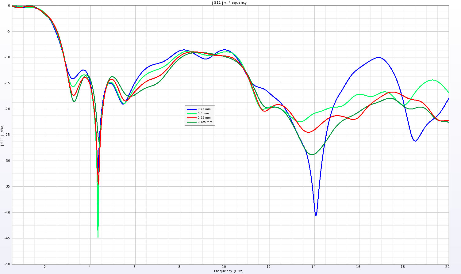
Figure 5: A comparison of the return loss for the antenna at four different cell sizes.
A secondary simulation is run with a 0.5 mm cell size that saves more output data including far field gain patterns and near field distribution images. This simulation uses 125 MB of memory and runs in about two minutes on an NVIDIA Quadro 3000M card.
First, the far field total gain at 10 GHz is plotted in three dimensions as shown in Figure 6, where the maximum gain of about 5 dBi is shown by the white arrow and the angular references Theta and Phi shown by blue and red arrows. The patterns in the Phi=0 degrees (plane of the antenna) direction are shown at 10 GHz in the line plots of Figure 7, while those in the Phi=90 degree (perpendicular to the plane of the antenna) are shown in Figure 8.
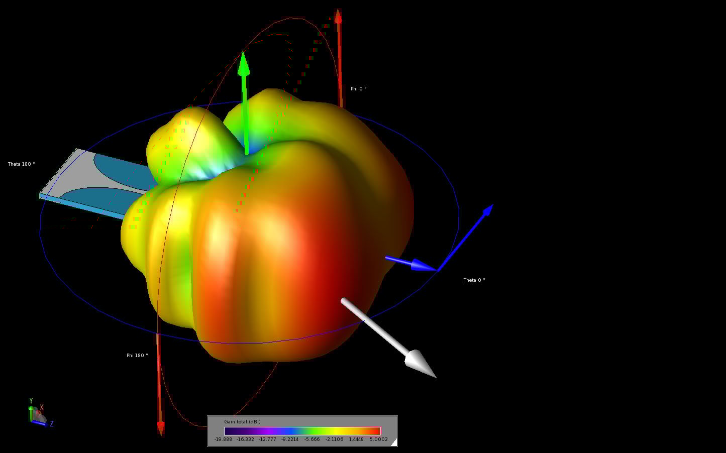
Figure 6: The three dimensional far field gain pattern of the antenna at 10 GHz with the maximum direction indicated by the white arrow and the angular references shown as blue (theta) and red (phi) arrows.
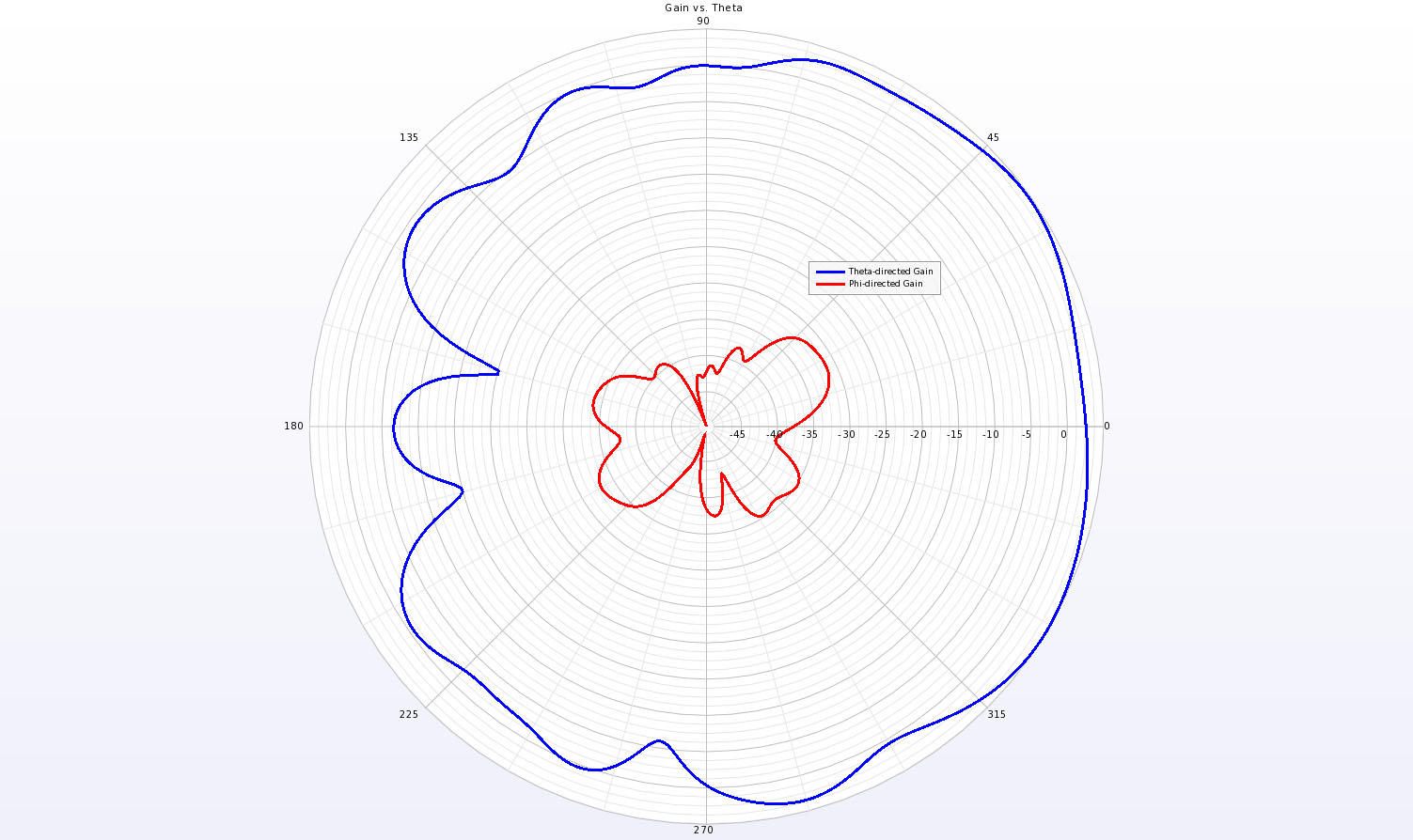
Figure 7: A polar plot of the gain in the Phi=0 plane (E-plane/plane of the antenna) at 10 GHz.
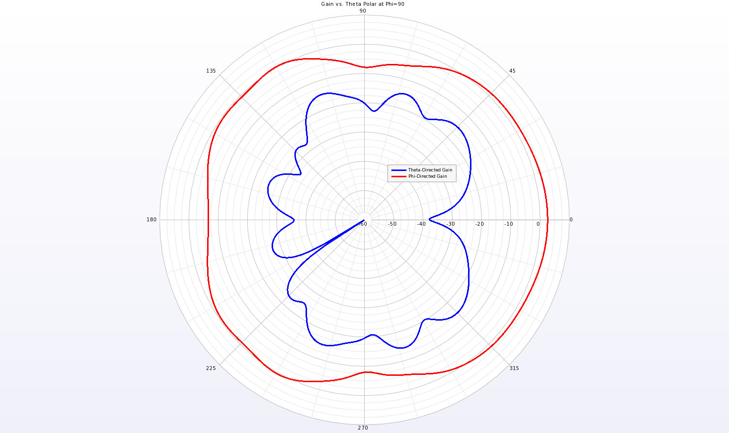
Figure 8: A polar plot of the gain in the Phi=90 plane (H-plane/perpendicular to the antenna) at 10 GHz.
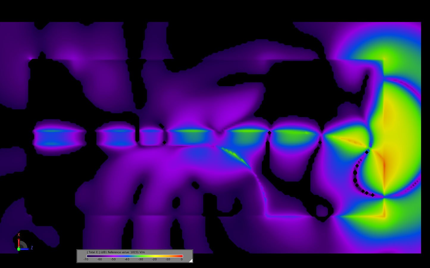
In Figures 9 and 10 the steady state current distribution is shown on the top and center conductors at 10 GHz. Figures 11 through 15 show the propagation of the transient electric field over the center of the antenna at five steps in time from the initial pulse entering the feed to the field radiating out of the end of the antenna.
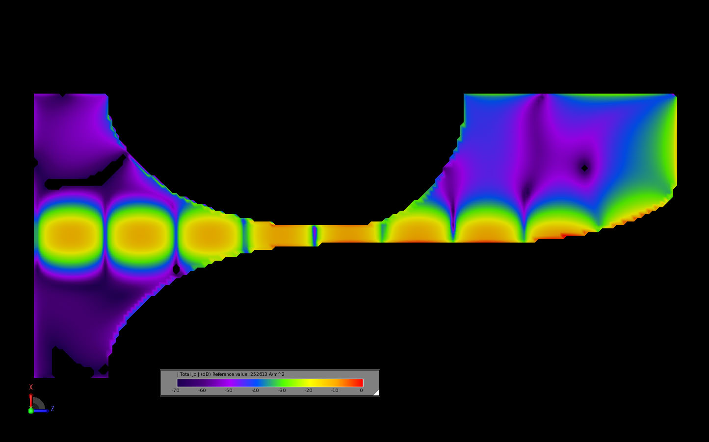
Figure 9: Steady state conduction currents on the outer element of the antenna at 10 GHz.
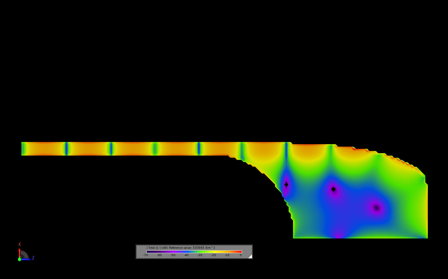
Figure 10: Steady state conduction currents on the outer element of the antenna at 10 GHz.
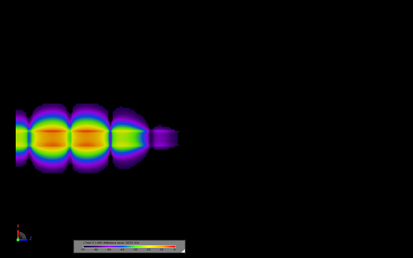
Figure 11: Transient electric field distribution at the center of the antenna at 0.314 ns.
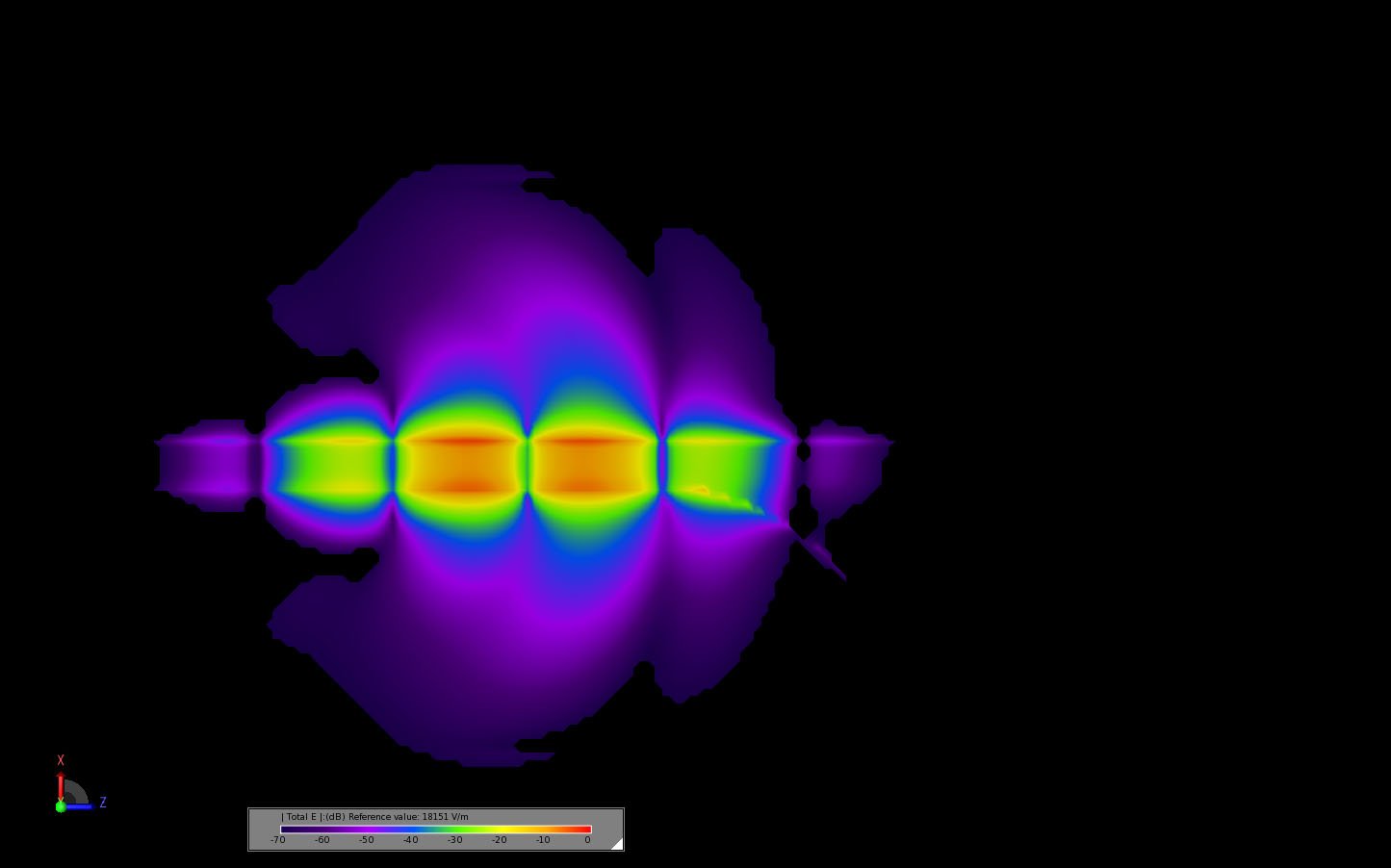
Figure 12: Transient electric field distribution at the center of the antenna at 0.419 ns.
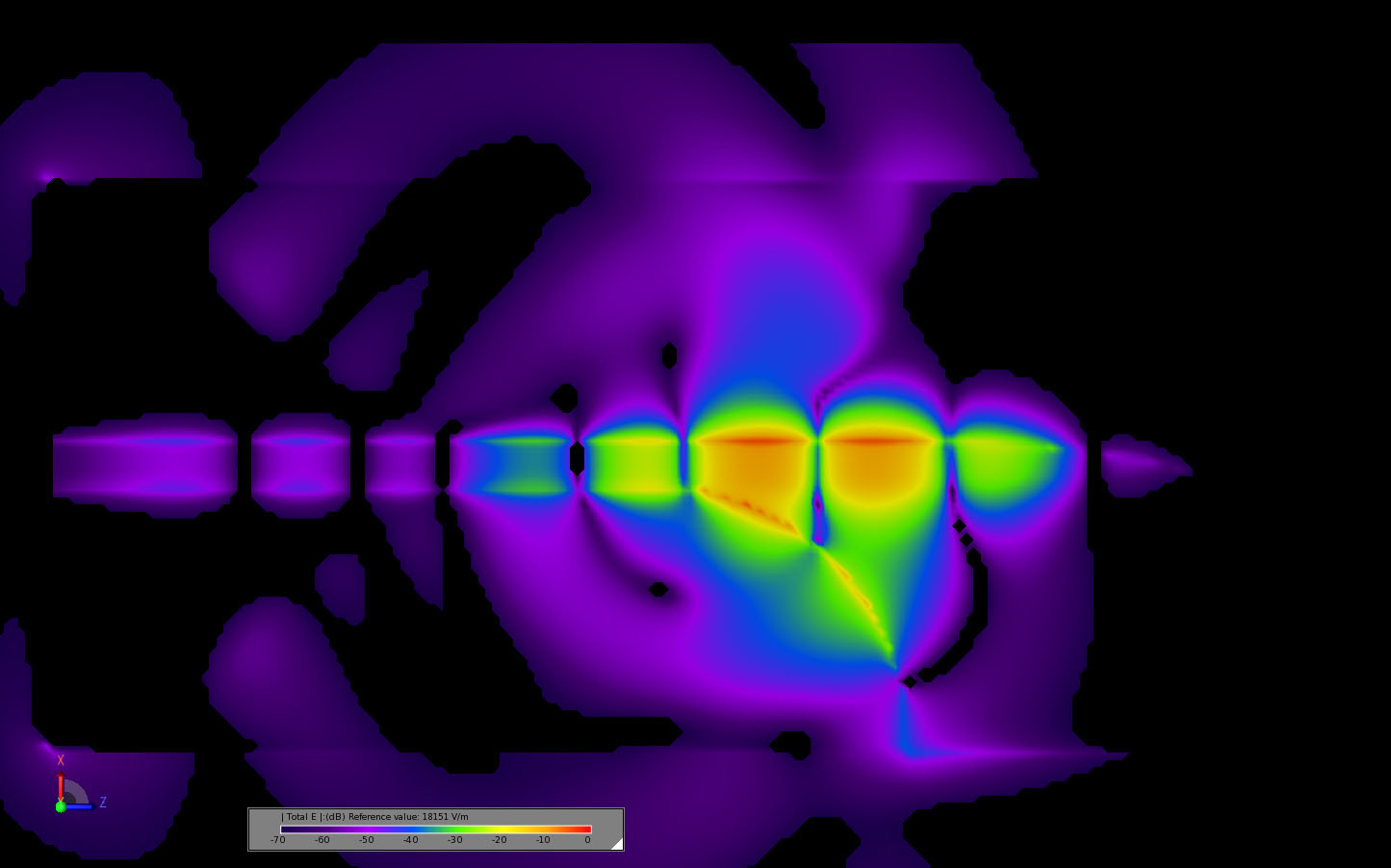
Figure 13: Transient electric field distribution at the center of the antenna at 0.524 ns.
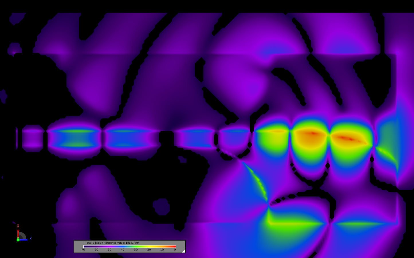
Figure 14: Transient electric field distribution at the center of the antenna at 0.628 ns.