With the need for real time propagation growing each day, a new way to simulate propagation models is needed that is closer to real time while maintaining the same amount of accuracy. The way to get the most accurate results is to use a high fidelity model such as a Finite Difference Time Domain (FDTD) model. This model is limited in space and computational resources. With the way the algorithm is calculated, the computational space can become massive very quickly. Therefore modeling long distances can be impossible. One way around that is to employ a method called Moving Window Finite Difference Time Domain (MWFDTD). This method only takes into account the area around the pulse. However, this is not close to real time due to computational intensity. One way to make this faster would be to make the calculations faster by using a Graphics Processor Unit (GPU). The GPU can be used to speed up the calculations like those found within MWFDTD.
Introduction
This paper discusses the challenges and techniques involved in converting the MWFDTD algorithm from a C++ implementation to an appropriate form for leveraging graphics processor units (GPUs) through NVIDIA’s CUDA framework. The GPU approach employs thousands of threads simultaneously which requires special design considerations in order to achieve maximum speedups. Previous work [1,2,3] has concentrated on the challenges of implementing GPU-targeted software through the use of the OpenGL API or the Cg language. With proper understanding of CUDA, it is possible to reach speedups of beyond two orders of magnitude over traditional CPUs and increase performance by a factor of two or more over previous GPU implementations.
Moving Window Finite Difference Time Domain
In order to model long range propagation using traditional 2D FDTD, a vertical plane containing the entire irregular terrain profile is projected onto a rectangular grid consisting of evenly spaced grid points in the x-y plane. In addition, time is divided into evenly spaced intervals. To begin the simulation, an electromagnetic pulse is excited at the transmitting antenna and at each time step, the electromagnetic fields at each grid point is determined by solving Maxwell’s equations using the second-order finite differencing method of Yee[4]. The MWFDTD propagation model is based on a modified FDTD to model radio wave propagation[5],[6].
One fact of a traditional FDTD method is the propagation radio pulse only occupies a small part of the computational space. MWFDTD takes advantage of this by limiting the computational space to the area surrounding the pulse. The window is only as wide and high as the pulse will be. All the other space in a traditional FDTD calculation could be considered as waste. This allows longer runs because the memory and time limitations are not as great. As the pulse propagates along the terrain, the FDTD mesh is moved forward to track the pulse as depicted in Figure 1. The window moves at the speed of light to follow the pulse that is also moving at the speed of light.
 Figure 1: Moving Window Finite Difference
The limited computational space does not compromise the accuracy of MWFDTD. MWFDTD is just as accurate as a regular FDTD calculation. "Error! Reference source not found." is the path loss calculated at a frequency of 410MHz, with a FDTD computational domain of 1000 cells wide by 4600 cells high, a cell spacing of 7.31 cm by 7.31 cm, which corresponds to 10 cells per wavelength at 410 MHz. The time step is chosen to be 0.181 ns. The results were compared with data obtained by ITS. The difference between MWFDTD and the measurements is at most 2-3 dB.
CUDA GPU
Once used for the sole purpose of driving graphical displays, the GPU has evolved into a powerful computational device. The Tesla C1060 offers a peak performance of 933 GFLOPS and a memory bandwidth of 102 GB/s. This can yield significant performance gains over even a 2.66 GHz Intel Core 2 Quad processor which has a theoretical peak performance of 42.56 GFLOPS (using all four cores and full SSE2 optimizations) and a memory bandwidth of 10.7 GB/s. The recently released Fermi C2050 and C2070 GPUs extend these differences even further with a peak performance of 1.03 Tflops and a memory bandwidth of 144 GB/s.
CUDA allows software developers to leverage this power without the need for special computer graphics knowledge [7][8]. The GPU is organized into a series of multiprocessors. Each of these multiprocessors contains a set of stream processors and a shared memory cache to facilitate thread cooperation.
CUDA compliant GPUs follow a single instruction multiple thread (SIMT) architecture [9]. In a SIMT model, threads are launched simultaneously in groups termed warps. Each thread in the warp can execute concurrently as long as they are performing the same instruction on different pieces of data. If threads of a warp diverge through a conditional branch, thread execution must be serialized. The greatest speed gains are achieved by designing software that minimizes thread divergence within a warp. Algorithms such as FDTD perform small amounts of work on large amounts of data, so memory bandwidth tends to be a critical factor in application performance. The GPU offers another significant advantage in this area. GPU threads can switch contexts nearly instantaneously - without the need to store and restore thread state. This fact allows the GPU to hide memory latency by launching thousands of threads simultaneously and performing rapid context swapping while waiting for input data.
Instantaneous context switching is important for hiding memory latency. CUDA devices offer several types of memory. The three most important types for these purposes are shared, constant, and device (global) memory. Shared memory is cached on chip memory with low latency that can be accessed cooperatively by a group of threads. It is particularly useful for implementing user defined caches. Constant memory is a cached read-only section of memory currently limited to 64 KB. Device or global memory is relatively high latency but is currently available in amounts up to 6 GB per device.
Implementation
Functions targeted for the GPU are implemented as kernels in CUDA. Kernels are very similar to C functions except there are certain extensions needed. This creates a very easy transition for a new user to implement any function using a kernel. The MWFDTD GPU library was written using a number of kernels to utilize the GPU.
The GPU kernels were used in the main update equations, boundary conditions and shifting the arrays as the window moves. These are the core FDTD functions within the MWFDTD function. Each of these functions required special consideration with regards to the MWFDTD implementation.
The first step was to convert the update equations from C to CUDA. This was done by converting the update functions to update kernel functions. The main task here was to eliminate the loop that was used within the equations. The kernel functions will loop over the data available without having the user implement a loop. The rest of the functions were then converted using the same idea.
The next step was to define all of the constant data like material identifiers, material constants, and all other constant arrays. This data will be needed at each time step and each time the window will move. There are two methods that CUDA capable GPU can read or write from/to global memory; coalesced and uncoalesced. Coalesced reads or writes allowed the GPU to perform memory transactions of 32, 64, or 128 bytes simultaneously. This is the most optimized what to read and write to a GPU due to the fact uncoalesced reads have to be serialized which could require between 400 and 600 clock cycles. The MWFDTD model utilized this fact by allocating the update coefficients in constant memory instead of global memory. This is due to the fact these needed to be read at every time step.
The last step was to implement the functions that will move the window. Each time the window moves new data has to be read into the problem, old data deleted, and all arrays have to be shifted. This was done utilizing various aspects of CUDA’s capability of shifting arrays within memory. The key was to minimize the number of reads from main memory. The reads were done while the results from the previous window were being written back to main memory. Also the number of reads were minimized by only reading in the new column of data and shifting the data that was already on the card.
To document the speedsup within the new MWFDTD model, simple test cases were developed to utilize the new GPU implementation of the model. Each test case was run first in the released MWFDTD 2.5 version and then rerun using the same setup file in the new GPU Implementation in 2.6 version. Results were then compared.
As with other FDTD methods, terrain type impacts scenario set up thus affecting runtimes. The terrain type impacts the number of cells per wavelength. The more cells present within the window, the longer the runtimes. Dry sand terrain scenarios run with 20 cells per wavelength while sea water terrain scenarios run with 100 cells per wavelength. 10 cells per wavelength in the material is needed. To find this value, Equation 1 is used. Table 2 shows a summary of the cells per wavelength per test.
 Equation 1
Each test case consists of a terrain defined by the terrain type at the set range. The waveform used a sinusoid with a carrier frequency defined in the Table 1. The antenna was an isotropic antenna with the defined waveform. There was one transmitter for each project. The number of receivers for each project is defined in the table.
 Figure 2: Example Project
The computer configuration for the tests is listed in Table 3.
Timing for a complete simulation was the benchmark used to evaluate the performance of the new MWFDTD model. Each of the tests described in Section 5 where first run using the CPU implementation then run on the same computer using the GPU implementation.
The speedup comparisons are depicted in Figure 3.
 Figure 3: Runtime Comparisons
Test 3 has the largest speedup due to the material that was used. This material required a denser grid. This denser grid creates the need for more calculations to be performed each time step. The GPU runtimes for this particular case are closer to the other cases. This is due to the fact the GPU can process the calculations simultaneously thus processing more data in a shorter amount of time. This shows the true power of the GPU.
 Figure 4: Speedup Comparisons
The speedups achieved are between 38X – 62X. The results show the more complex problems benefit the most from the new GPU implementation. The Wet Earth test cases shows the highest speedup due to the materials used, the range of the problem, and the frequency of the antenna. The sea water case has a lot of cells in each window which results in a long runtime. The majority of the GPU runtimes are very similar as opposed to the CPU runtimes which are all over the board. This is due to the fact the GPU can simultaneously calculate hundreds of grid points while the CPU is limited on the amount of calculations it can perform. This allows most if not all of the cells in one vertical column to be calculated at once instead of one or maybe two at a time like on the CPU thus resulting in the same runtimes for each column. Due to the ability to only calculate one column at a time, the GPU has enough memory to calculate the denser grids like in the wet earth test case in similar time as the less dense grid test case.
MWFDTD was an ideal program to port over to the GPU. The calculations are able to be performed in parallel to completely utilize the power of the GPU.
References
-
M. J. Inman, A. Z. Elsherbeni, and C. E. Smith “GPU Programming for FDTD Calculations,” The Applied Computational Electromagnetics Society (ACES) Conference, Honolulu, Hawaii, 2005.
-
M. J. Inman and A. Z. Elsherbeni, “3D FDTD Acceleration Using Graphical Processing Units,” The Applied Computational Electromagnetics Society (ACES) Conference, Miami, Florida, 2006.
-
Adams, Samuel, Jason Payne, and Rajendra Boppana, “Finite Difference Time Domain (FDTD) Simulations Using Graphics Processors”, HPCMP Users Group Conference, 2007
-
K. S. Yee, “Numerical solution of initial boundary value problems involving Maxwell’s equations in isotropic media,” IEEE Trans. Antennas Propagat., vol. 14, pp. 302-307, 1966.
-
Luebbers, R.; Schuster, J.; Wu, K., "Full wave propagation model based on moving window FDTD," Military Communications Conference, 2003. MILCOM 2003. IEEE , vol.2, no., pp. 1397-1401 Vol.2, 13-16 Oct. 2003
-
M. F. Hadi and M. Piket-May, “A modified FDTD (2,4) scheme for modeling electrically large structures with high-phase accuracy,” IEEE Trans. Antennas Propagat. vol. 45, pp. 254-264, 1997.
-
Lindholm, E., Nickolls, J., Oberman, S., and Montrym, J. “NVIDIA Tesla: A Unified Graphics and Computing Architecture,” IEEE Micro 28, pp. 39-55, March 2008.
-
Nickolls, J., Buck, I., Garland, M., and Skadron, K., “Scalable Parallel Programming with CUDA,” Queue 6, pp. 40-53, March 2008.
-
“CUDA Programming Guide, 2.1,” NVIDIA